Topics in Quantitative Finance, Summer 2025

Lecture 6: Optimal execution under price impact

Tai-Ho Wang (王太和)

\[ \newcommand{\bea}{\begin{eqnarray}} \newcommand{\eea}{\end{eqnarray}} \newcommand{\supp}{\mathrm{supp}} \newcommand{\F}{\mathcal{F} } \newcommand{\cF}{\mathcal{F} } \newcommand{\cG}{\mathcal{G} } \newcommand{\E}{\mathbb{E} } \newcommand{\Eof}[1]{\mathbb{E}\left[ #1 \right]} \newcommand{\Etof}[1]{\mathbb{E}_t\left[ #1 \right]} \def\Cov{{ \text{Cov} }} \def\Var{{ \text{Var} }} \newcommand{\1}{\mathbf{1} } \newcommand{\p}{\partial} \newcommand{\PP}{\mathbb{P} } \newcommand{\Pof}[1]{\mathbb{P}\left[ #1 \right]} \newcommand{\QQ}{\mathbb{Q} } \renewcommand{\R}{\mathbb{R} } \newcommand{\DD}{\mathbb{D} } \newcommand{\HH}{\mathbb{H} } \newcommand{\spn}{\mathrm{span} } \newcommand{\cov}{\mathrm{cov} } \newcommand{\HS}{\mathcal{L}_{\mathrm{HS}} } \newcommand{\Hess}{\mathrm{Hess} } \newcommand{\trace}{\mathrm{trace} } \newcommand{\LL}{\mathcal{L} } \newcommand{\s}{\mathcal{S} } \newcommand{\ee}{\mathcal{E} } \newcommand{\ff}{\mathcal{F} } \newcommand{\hh}{\mathcal{H} } \newcommand{\bb}{\mathcal{B} } \newcommand{\dd}{\mathcal{D} } \newcommand{\g}{\mathcal{G} } \newcommand{\half}{\frac{1}{2} } \newcommand{\T}{\mathcal{T} } \newcommand{\bit}{\begin{itemize}} \newcommand{\eit}{\end{itemize}} \newcommand{\beq}{\begin{equation}} \newcommand{\eeq}{\end{equation}} \newcommand{\tr}{\text{tr}} \renewcommand{\underbar}{\underline} \newcommand{\mbA}{\mathbf A} \newcommand{\mbB}{\mathbf B} \newcommand{\mbP}{\mathbf P} \newcommand{\mbQ}{\mathbf Q} \newcommand{\mbR}{\mathbf R} \newcommand{\mbS}{\mathbf S} \newcommand{\bA}{\boldsymbol A} \newcommand{\bB}{\boldsymbol B} \newcommand{\bu}{\boldsymbol u} \newcommand{\bq}{\boldsymbol q} \newcommand{\bW}{\boldsymbol W} \newcommand{\bX}{\boldsymbol X} \newcommand{\bx}{\boldsymbol x} \newcommand{\bSigma}{\boldsymbol \Sigma} \newcommand{\tS}{\tilde S} \newcommand{\inn}[2]{\left\langle #1, #2 \right\rangle} \]

Agenda

Market impact of meta orders
- Impact profile
Empirical market impact profiles
Optimal execution as variational and control problems
- risk neutral
- mean-qv optimization
The Almgren-Chriss model and the Almgren-Chriss optimal liquidation strategy (Almgren and Chriss 2001)
The Obizhaeva-Wang model (Obizhaeva and Wang 2013)
Combining Almgren-Chriss and Obizhaeva-Wang: the ACOW model
- Numerical examples

What is market or price impact?

Empirically, in average a buy order pushes the price up whereas a sell order sends the price down. This empirically observed market phenomenon is referred to as price impact of transaction or trading.

A price impact model is a model aiming at quantify the relationship between the transacted volume and price.

The square-root formula for market impact

For many years, traders have used the simple sigma-root-liquidity model described for example by Grinold and Kahn in 1994.
Software incorporating this model includes:
- Salomon Brothers, StockFacts Pro since around 1991
- Barra, Market Impact Model since around 1998
- Bloomberg, TCA function since 2005
The model is always of the rough form
\[\Delta P = \text{Spread cost} +\alpha\,\sigma\,\sqrt{\frac Q V}\] where $\sigma$ is daily dollar volatility, $V$ is daily volume, $Q$ is the number of shares to be traded and $\alpha$ is a constant pre-factor of order one.

注: Spread. 在金融市场中, 资产通常有两个报价:

Bid price (买入价): 交易者愿意支付的价格
Ask price (卖出价): 交易者愿意接受的价格

这两者之间的差额就是 Spread (点差).

注: Spread cost. 无论你买入还是卖出, 你都会吃掉一半的 spread. 也即市场的合理参考价应该为 Mid price, 但是你买入的时候, 一般成交价为 Best Ask, 这和 Mid price 有差距, 这部分差距就是 Spread cost. 同理, 卖出的时候, 一般成交价为 Best Bid, 这和 Mid price 有差距, 这部分差距也是 Spread cost. \[ \text{Spread cost} = \frac{1}{2} \times \text{Spread} \]

Commonly applied algorithms

VWAP “Volume weighted average price”
- Trades at constant rate in volume time
POV “Percentage of volume”
- Participate at a certain percentage of market volume
TWAP “Time weighted average price”
- Trades at constant rate in wall clock time
IS “Implementation shortfall”
- Trades faster at the beginning and more slowly at the end
- To balance the risk of a worse price against the benefit of better execution from being patient.

注: 当你需要执行一个较大的订单, 不希望对市场价格造成太大影响, 你可以使用一些算法来分批执行这个订单, 以降低市场冲击.

算法	执行方式	优点	缺点	适用场景
VWAP	与当天成交量历史分布挂钩	平衡性好、易控风险	无实时感知、不区分价格趋势	流动性高、全天相对均衡的市场
POV	实时按市场成交量比例自动下单	实时自适应, 部分规避流动性脉冲	需要准确设置参与率、易触发极端执行	市场节奏多变、成交量波动大时
TWAP	时间切片均等、无视成交量	简单易理解, 执行控制明确	在低晶流动性时间段易导致更差执行价格	流动性波动大、但对价格执行节奏敏感时
IS	前期迅速、后期委细	最好控制决策价偏离, 较兼顾速度与成本	有执行风险, 受市场判断影响大	对价格走势敏感、需尽快完成交易时

Terminology

Metaorder means that a sufficiently large order that cannot be filled immediately without eating into the order book.
- Such orders need to be split.
- Each component of a metaorder is referred to as a child order.
The impact profile refers to the average path of the stock price during and after execution of a metaorder.
Completion refers to the timestamp of the last executed child order.

Schematic of impact profile

The impact profile

Stylized features of impact profile

When a buy metaorder of length $T$ is sent, its immediate effect is to move the price upwards (to $S_T$ say).
After completion, the price reverts to some price $S_{\infty}$ (which may be the starting price $S_0$).
Market impact thus has two components: one transient and one permanent.
Knowledge of the metaorder impact profile is key to the derivation of optimal execution strategies.

Empirical market impact profiles from (Bacry et al. 2014)

Empirical market impact profiles from (Zarinelli et al. 2014)

Notations

The following notations will be used throughout.

$S_t$: mid or efficient price
$\tilde S_t$: transaction price. Thus, $\tilde S_t = S_t + \text{spread}$.
$\sigma$: volatility of stock.
$Z_t$: Brownian motions
$v_t$: trading rate at time $t$
$X_t$: remaining orders to be executed at time $t$

Almgren and Chriss

Almgren and Chriss treats the execution of a meta order as a tradeoff between risk and execution cost.
According to their formulation:
- The faster an order is executed, the higher the execution cost
- The faster an order is executed, the lower the risk (which is increasing in position size).
Note that this is inconsistent with the empirical success of the square-root formula in describing the cost of meta orders.

The price impact model of Almgren and Chriss

For simplicity, we consider liquidation of an existing position $X$. Denote the position at time $t$ by $x_t$ with $x_0=X$ and $x_T=0$.

Almgren and Chriss model market impact and slippage as follows.

\[ \tilde{S}_t = S_t + \eta v_t = s_0 + \sigma_S Z_t + \gamma(X_t - x_0) + \eta v_t, \]

where $\displaystyle X_t = x_0 + \int_0^t v_s \mathrm{d}s$.

注:

$s_0$: 清仓前的价格
$\sigma_S Z_t$: 无冲击的随机价格波动
$\gamma (X_t - x_0)$: 永久性冲击, 也即清仓后价格的变化. 由于你累积卖出 (或买入) 所带来的永久 (permanent) 价格冲击
$\eta v_t$: 临时性冲击, 瞬时提交量导致的影响.

\[\begin{align*} \Eof{\tilde{S}_t - s_0} &= \sigma_S \Eof{Z_t} + \gamma \Eof{X_t - x_0} + \eta \Eof{v_t} \\ &= \gamma \int_0^t v_s \mathrm{d}s + \eta v_t. \end{align*}\]

Note

$\eta v_t$: temporary impact
$\gamma (X_t - x_0)$: permanently impact
$X_t = x_0 + v t$ if $v_t \equiv v$, a constant.

Suppose $\displaystyle v_t = - \frac{x}{T}$, then: \[ \Eof{\tilde{S}_t - s_0} = \gamma x \left( 1 - \frac{t}{T} \right) + \eta \frac{x}{T}. \]

Impact profile in the Almgren and Chriss model

import numpy as np
import matplotlib.pyplot as plt

T = 1
vwap_AC = lambda t: t/T*(t <= T) + T*(t > T)
t = np.linspace(0, 2, 200)
#plt.figure(figsize=(8, 6))
plt.plot(t, vwap_AC(t), color='orange', label='Almgren-Chriss')
plt.vlines(x=1, ymin=0, ymax=2, linewidth=0.5, ls='dotted')
plt.ylim([0, 1.5])
plt.xlabel(r'$t$', fontsize=15)
plt.ylabel(r'$\mathbb{E}|S_t - S_0|$', fontsize=15)
plt.title('Almgren-Chriss price path', fontsize=18);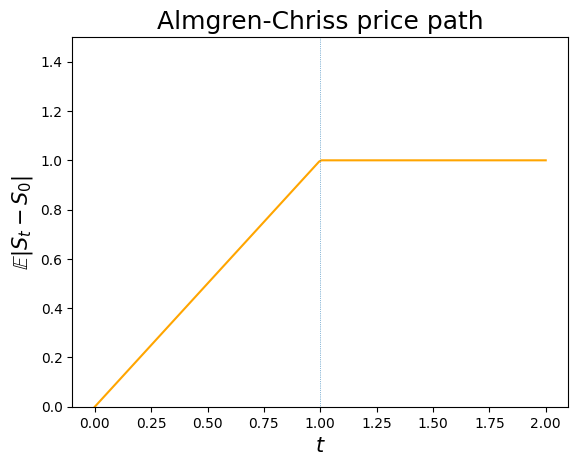

Inconsistency with empirical observation

This price path is inconsistent with empirical observation:
- The average price path during execution is linear.
- There is no price reversion after completion of the order.

P&L and cost of trading of a trading strategy

Let $x_t$ be a trading strategy. The corresponding P&L (up to time $t$), denoted by $\Pi_t(x)$, is identified as

\[ \Pi_t(x) := x_t (S_t - S_0) + \int_0^t (S_0 - \tilde S_\tau) \mathrm{d} x_\tau. \]

The first term represents the (fair) value of stock shares that are yet to be transacted.
The second term corresponds to the monetary value collected from the shares that have been transacted up to time $t$. 也就是, 在时刻 $\tau$ 以 $\tilde S_\tau$ 的价格成交的股票, 但是参考价为 $S_0$, 你已经收到了 $(S_0 - \tilde S_\tau)$ 的 P&L.
Obviously, should there be no trade in the time interval $[0,t]$, i.e., $x_s = X$ for all $s \in [0,t]$, the P&L reads $\Pi_t(x) = X (S_t - S_0)$; reflecting the P&L from the price movement of the stock.

Implementation shortfall as cost of trading

Negative P&L is also referred to as the implementation shortfall, which will be used as the cost of trading, denoted by $C$ hereafter. 对于一个 trading strategy $x$, 如果它的 P&L 为 $\Pi_t(x)$, 那么它的交易成本为 $C(x) = - \Pi_t(x)$.

P&L in Almgren-Chriss model

Note that, at the end of execution period $T$, the P&L reads \[ \Pi_T(x) = x_T (S_T - S_0) + \int_0^T (S_0 - \tilde S_u) \mathrm{d} x_u, \] should there be $x_T$ shares yet to be transacted. Hence, in Almgren-Chriss model

\[\begin{align*} \Pi_T(x) &= x_T (S_T - S_0) + \int_0^T (S_0 - \tilde S_u) \mathrm{d} x_u \\ &= \int_0^T [- \gamma (x_u - X) - \sigma Z_u - \eta v_u] \mathrm{d} x_u \quad (\text{note that } x_T = 0) \\ &= -\frac\gamma2 X^2 + \sigma \int_0^T x_u \mathrm{d} Z_u - \eta \int_0^T v_u^2 \mathrm{d} u \quad (\text{Integration by parts}). \end{align*}\]

Therefore, the expected cost corresponding to the trading strategy $x$ is given by

\[\begin{align*} & \E\left[C_T(x)\right] = \E\left[-\Pi_T(x)\right] = \frac\gamma2 X^2 + \eta \int_0^T \Eof{v_u^2} \mathrm{d} u. \end{align*}\]

Expected cost of TWAP in the Almgren and Chriss model

For a TWAP, $\displaystyle v_t = -\frac XT$ where $X$ is the total trade size and $T$ is the duration of the order.

注: TWAP (Time Weighted Average Price) 是一种交易策略, 它在整个交易期间内以恒定的速率执行订单, 以避免对市场价格造成过大的冲击. 它对应的公式为:

\[ v_t = -\frac{X}{T}, \] 然后把这个替换入 Almgren-Chriss 模型的公式中.

Then, we have

\[\begin{align*} \E[C_T(x)] &= \frac\gamma2 X^2 + \eta \int_0^T \left(\frac XT\right)^2 \mathrm{d} u \\ &= \frac\gamma2 X^2 + \eta \frac{X^2}T \\ &= \left(\frac\gamma2 + \frac\eta{T}\right)X^2. \end{align*}\]

The cost per share $\hat C$ of executing an order using TWAP is therefore

\[\hat{C}=\left(\frac\gamma2 + \frac\eta{T}\right)X\]

which is linear in the trade size $X$ and inversely proportional to the duration of the order.

Optimal strategy of a risk neutral trader

For a risk neutral trader whose objective is to minimize the cost of trading, the optimal control problem reads

\[\begin{align*} & \min_{v} \E\left[C_T(x)\right] \\ &= \min_{v} \left\{\frac\gamma2 X^2 + \eta \int_0^T \Eof{v_u^2} \mathrm{d} u \right\} \\ &= \frac\gamma2 X^2 + \eta \min_v \int_0^T \Eof{v_u^2} \mathrm{d} u, \end{align*}\]

where the state variable $x_t$ is driven by $\mathrm{d} x_t = v_t \mathrm{d} t$ with the constraints $x_0 = X$ and $x_T = 0$.
Note that, since $S_t$ is not involved in the last expression, we end up with a deterministic control problem which can be solved by the solution to its associated HJB equation or, due to the simplicity of the dynamics of $x_t$, further reduced to a variational problem.

注: risk-neutral trader 表示: Risk neutral investors may understand that risk is involved, but they aren’t considering it for the moment. 可以理解为完全不考虑 $S_t$ 的价格波动影响, 只考虑交易成本.

Quotes from Investopedia:

Risk neutral is a term used to describe the attitude of an individual who may be evaluating investment alternatives. If the individual focuses solely on potential gains regardless of the risk, they are said to be risk neutral. Such behavior, to evaluate reward without thought to risk, may seem to be inherently risky. A risk averse investor would not consider the choice to risk a $1000 loss with the possibility of making a $50 gain to be the same as risking only $100 to make the same $50 gain. However someone who is risk neutral would. Given two investment opportunities the risk-neutral investor only looks at the potential gains of each investment and ignores the potential downside risk.

Variational problem

\[\min_x \int_0^T\,\dot x_t^2\,\mathrm{d}t\]

with $v_t=\dot x_t$ and $x_0 = X$, $x_T = 0$.

The Euler-Lagrange equation is then

\[\partial_t v_t=\partial_t^2 x_t=0\]

with boundary conditions $x_0=X$ and $x_T=0$ and the solution is obviously

\[v_t = -\frac{X}{T}; \, x_t=X\,\left(1-\frac{t}{T}\right)\]

注: 想象成一个最小化能量的问题, 那么就是沿着直线走.

注: Euler-Lagrange 方程是变分问题中的一个方程, 它是泛函达到极值 (严格地说, 是临界值) 的一个必要条件, 其地位类似于多元函数中梯度为零在极值分析中的地位.

假设求解泛函的函数空间为: \[ M = \{u \in C^1([t_0,t_1] \to U \subset \R^N): u(t_0) = P_0 \in U, u(t_1) = P_1 \in U\}, \] (其实, $U$ 就是 $u$ 的值域). 定义一个连续可微的函数:

\[\begin{align*} L: [t_0,t_1] \times U \times \R^N &\to \R, \\ (t,u,p) &\mapsto L(t,u,p). \end{align*}\]

这里的 $p$ 一般代表 $u$ 的导数, 即 $p = \dot u$. 那么, 泛函的形式为:

\[ I(u) = \int_{t_0}^{t_1} L(t,u(t),\dot u(t)) \mathrm{d} t. \]

那么该泛函的极值 $u^*$ 满足如下 Euler-Lagrange 方程:

\[ \int_{t_0}^t L_{u^i} (s, u(s), \dot u(s)) \mathrm{d} s + L_{p^i} (t, u(t), \dot u(t)) = C_i, \quad i=1,\ldots,N, \]

注: 如果 $L,u$ 是 $C^2$ 的, 那么上述积分形式的关系式可以求导: \[ - \frac{\mathrm{d}}{\mathrm{d} t} L_{p^i} (t, u(t), \dot u(t)) + L_{u^i} (t, u(t), \dot u(t)) = 0, \quad i=1,\ldots,N. \]

注: 我们现在假设 $N=1$, 且此时 Euler-Lagrange 方程不含有 $u$, 此时有下面的形式:

\[ \frac{\mathrm{d}}{\mathrm{d} t} L_{p} (t, \dot u(t)) = 0. \]

注: 如果不含有 $p$ 的话, 那么 Euler-Lagrange 方程的形式为: \[ L_{u} (t, u(t)) = 0. \] 这是一个常微分方程.

Risk neutral trader: TWAP is optimal in Almgren-Chriss

As naive as the TWAP strategy may look, it is indeed optimal for a risk neutral trader in the Almgren-Chriss model.

注: TWAP: Time Weighted Average Price, refer to Commonly applied algorithms.

Penalty by quadratic variation

Almgren and Chriss^[2] add a risk term that penalizes the approximate variance of the trading cost. They claim

\[ \text{Var} \left[\int_0^T\,x_t\,\mathrm{d} S_t\right] \approx \sigma^2\,\int_0^T\,x_t^2\,\mathrm{d} t. \]

In fact, by Itô’s isomety, it is an equality if $x_t$ is deterministic.

The expected risk-adjusted cost is then given by (temporarily ignore the path independent term $\displaystyle \frac\gamma2 X^2$)

\[\eta\,\int_0^T\,{\dot x}_t^2\,\mathrm{d}t + \lambda\,\sigma^2\,\int_0^T\,x_t^2\,\mathrm{d}t\]

for some price of risk $\lambda$.

Note the analogies to physics and portfolio theory.
- The first term looks like kinetic energy and the second term like potential energy.
- The expression looks like the objective in mean-variance portfolio optimization.

注: 写成泛函的形式, $L(t, x(t), {\dot x}(t)) = \eta {\dot x}^2(t) + \lambda \sigma^2 x^2(t)$. 那么现在的 Euler-Lagrange 方程为: \[ \frac{\partial L}{\partial x} - \frac{\mathrm{d}}{\mathrm{d} t} \frac{\partial L}{\partial {\dot x}} = 0. \]

The Euler-Lagrange equation becomes

\[\ddot x- \kappa^2\,x=0\]

with

\[\kappa^2=\frac{\lambda\,\sigma^2}{\eta}.\]

The solution is a linear combination of terms of the form $e^{\pm \kappa t}$ that satisfies the boundary conditions $x_0=X$, $x_T=0$.

注: 也就是说 \[ x(t) = A e^{\kappa t} + B e^{-\kappa t}, \] where $A$ and $B$ are determined by the boundary conditions.

Mean-QV trader: The Almgren-Chriss strategy

For risk averse traders, by using the quadratic variation of P&L during execution to penalize the terminal P&L/trading cost, the following strategy, referred to as the Almgren-Chriss strategy, is optimal.

\[ x(t) = X\,\frac{\sinh \kappa (T-t)}{\sinh \kappa T}, \]

where $\displaystyle \kappa = \sqrt{\frac{\lambda\sigma_S^2}\eta}$, $\lambda$ is the parameter that proxies the trader’s risk aversion.

注: \[ \sinh x = \frac{e^x - e^{-x}}{2}. \]

Note

The strategy is deterministic.
Almgren-Chriss strategy gives an example of Implementation Shortfall type: trade fast at the beginning and more slowly towards the end.

# order execution horizon
T = 1

# number of shares to execute
X = 10_000

# the Almgren-Chriss strategy
opt_AC = lambda t, kappa: X*np.sinh(kappa*(T - t))/np.sinh(kappa*T)

# plot
t = np.linspace(0, T, 100)
plt.figure(figsize=(8, 5))
for kappa in np.arange(1, 6):
    plt.plot(t, opt_AC(t, kappa), label=f'$\kappa$={kappa}')
    
plt.title('Almgren-Chriss strategy for various $\kappa$')
plt.xlabel(r'$t$')
plt.ylabel(r'$x$')
plt.legend();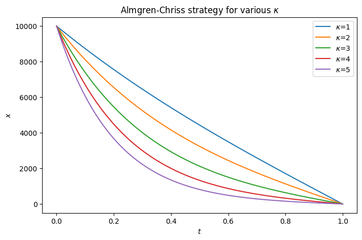

Applications of the Almgren-Chriss framework

Although the Almgren and Chriss price process is not particularly realistic, it leads to a tractable framework for solving a number of interesting practical problems.
Applications include:
- Portfolio liquidation
- Optimal liquidation with a dark pool (e.g. [Kratz and Schöneborn]^[7])
- Optimal delta-hedging of options under transactions costs (e.g. [Li and Almgren]^[8])
- Optimal liquidation in the presence of a trading signal (e.g. [Almgren(2012)]^[3])

Summary on the Almgren-Chriss model

The Almgren-Chriss price process is in practice the most widely-used.
It forms the basis for many of the algorithms and most of the thinking in algorithmic execution.
- despite the fact that it is unrealistic: market impact decays instantaneously and it is completely incompatible with the square-root law.
Because of the analytical tractability of the Almgren-Chriss framework, there are closed-form or quasi-closed-form solutions for many problems of practical interest.

Transient impact models

The price process assumed in transient impact model is

\[S_t = S_0 + \int_0^t\,h(v_s)\,G(t-s)\,\mathrm{d}s+M_t, \quad \text{ where } M_t \text{ is a zero mean martingale/noise.}\]

$h(v_s)$ is referred to as the instantaneous market impact function, which represents the impact of trading at time $s$, and $G(t-s)$ is a decay factor. Note that $h(v) > 0$ if $v > 0$; whereas $h(v) < 0$ if $v < 0$.
The cumulative impact of (others’) trading is implicitly in $S_0$ and the noise term.
The model is a generalization of processes due to Almgren, Bouchaud, and Obizhaeva and Wang.

Note

Transient impact model: 瞬态冲击模型.
$M_t$ 是一个零均值的鞅, 也即 $M_t$ 的期望为零, 它代表了市场噪音. 指交易对手或市场其他参与者的买卖行为引入的随机价格变动, 不由控制者交易产生
$h(v_s)$ 是瞬时市场冲击函数, 它表示在时间 $s$ 交易对市场价格的影响. 例如, 如果 $v_s > 0$, 那么 $h(v_s) > 0$, 表示买入对价格有正向影响; 如果 $v_s < 0$, 那么 $h(v_s) < 0$, 表示卖出对价格有负向影响.
$G(t-s)$ 是一个衰减函数, 它表示交易对价格的影响随时间的衰减. 例如, 如果 $G(t-s)$ 随着 $t-s$ 的增大而减小, 那么表示交易的影响会随着时间的推移而减弱.

P&L and cost of trading in transient impact model

\[\begin{align*} \Pi_T(x) &= x_T (S_T - S_0) + \int_0^T (S_0 - \tilde S_u) \mathrm{d} x_u \\ &= - \int_0^T \int_0^t h(v_u)G(t-u) \mathrm{d} u \mathrm{d} x_t - \int_0^T M_t \mathrm{d} x_t \quad (\text{since } x_T = 0) \\ &= - \int_0^T \int_0^t h(v_u)G(t-u) \mathrm{d}u \mathrm{d} x_t - (M_T x_T - M_0 x_0) + \int_0^T x_t \mathrm{d} M_t \quad (\text{Integration by parts}) \\ &= - \int_0^T \int_0^t h(v_u)G(t-u) \mathrm{d}u \mathrm{d} x_t + \int_0^T x_t \mathrm{d} M_t \quad (\text{since } x_T = 0 \text{ and } M_0 = 0). \end{align*}\]

Therefore, the expected cost corresponding to the trading strategy $x$ is given by

\[\begin{align*} & \E\left[C_T(x)\right] = \E\left[-\Pi_T(x)\right] = \Eof{\int_0^T \int_0^t h(v_u)G(t-u) \mathrm{d}u \mathrm{d} x_t}. \end{align*}\]

The optimal strategy of a risk neutral trader

For a risk neutral trader whose objective is to minimize the expected cost of trading, the optimal control problem reads

\[\begin{align*} & \min_{v} \E\left[C_T(x)\right] = \min_v \int_0^T \int_0^t h(v_u)G(t-u) \mathrm{d}u \mathrm{d} x_t, \end{align*}\]

where the state variable $x_t$ is driven by $\mathrm{d}x_t = v_t \mathrm{d}t$ with the constraints $x_0 = X$ and $x_T = 0$. It is equivalent to a variational problem.

\[\begin{align*} & \min_{v} \E\left[C_T(x)\right] = \min_v \left\{\int_0^T \int_0^t h(v_u)G(t-u) \mathrm{d}u v_t \mathrm{d}t\right\}, \end{align*}\]

subject to the constraint $\displaystyle \int_0^T v_t \mathrm{d}t = X$.

Lagrange multiplier

To derive the Euler-Lagrange equation, consider the Lagrangian

\[\begin{align*} & L(v,\lambda) = \int_0^T\int_0^t v_t G(t-s) h(v_s) \mathrm{d}s \mathrm{d}t - \lambda \left( \int_0^T v_t \mathrm{d}t - X \right) \\ &= \int_0^T \left[ \int_0^t G(t-s) h(v_s) \mathrm{d}s - \lambda \right] v_t \mathrm{d}t + \lambda X, \end{align*}\]

where $\lambda$ is the Lagrange multiplier.

Euler-Lagrange equation

Let $\varphi$ be a perturbation(扰动). Consider the first order criterion for the Lagrangian $L$:

\[\begin{align*} 0 &= \left.\frac{\mathrm{d}}{\mathrm{d}\epsilon}\right|_{\epsilon=0} L( v_t + \epsilon \varphi_t,\lambda) \\ &= \left.\frac{\mathrm{d}}{\mathrm{d}\epsilon}\right|_{\epsilon=0} \int_0^T \left[ \int_0^t G(t-s) h(v_s + \epsilon \varphi_s) \mathrm{d}s - \lambda \right] (v_t + \epsilon \varphi_t ) \mathrm{d}t \\ &= \int_0^T \left[ \int_0^t G(t-s) h'(v_s) \varphi_s \mathrm{d}s \right] v_t \mathrm{d}t + \int_0^T \left[ \int_0^t G(t-s) h(v_s) \mathrm{d}s - \lambda \right] \varphi_t \mathrm{d}t \\ &= \int_0^T \int_0^t G(t-s) h'(v_s) \varphi_s v_t \mathrm{d}s \mathrm{d}t + \int_0^T \left[ \int_0^t G(t-s) h(v_s) \mathrm{d}s - \lambda \right] \varphi_t \mathrm{d}t \\ % &= \int_0^T \int_s^T G(t-s) h'(v_s) \varphi_s v_t \mathrm{d}t \mathrm{d}s + \int_0^T \left[ \int_0^t G(t-s) h(v_s) \mathrm{d}s + \lambda \right] \varphi_t \mathrm{d}t \\ &= \int_0^T \left[ \int_t^T G(s-t) h'(v_t) v_s \mathrm{d}s + \int_0^t G(t-s) h(v_s) \mathrm{d}s - \lambda \right] \varphi_t \mathrm{d}t. \end{align*}\]

Since $\varphi_t$ is arbitrary (because the first order criterion must hold for any perturbation), we must have

(2) \[ \int_t^T G(s-t) h'(v_t) v_s \mathrm{d}s + \int_0^t G(t-s) h(v_s) \mathrm{d}s = \lambda \]

for all $0\leq t\leq T$. This is a generalized Fredholm integral equation of the first kind. The Lagrange multiplier $\lambda$ is determined by the constraint $\displaystyle \int_0^T v_t \mathrm{d}t = -X$.

The Obizhaeva and Wang model

The model in [Obizhaeva and Wang]^[7] is given by

(1) \[S_t = S_0 + \eta\,\int_0^t\,v_s\,e^{-\rho\,(t-s)}\,\mathrm{d}s + \sigma_S Z_t\]

with $v_t=\dot x_t$.

Market impact decays exponentially, i.e., $G(\tau) = e^{-\rho\tau}$
Instantaneous market impact is linear in the rate of trading, $h(v) = \eta v$.

The expected cost of trading becomes: \[\mathcal{C} =\eta\,\int_0^T\int_0^t\,{v}_s\,e^{-\rho\,(t-s)}\,\mathrm{d}s\, v_t\mathrm{d}t\]

Impact profile in the Obizhaeva and Wang model

rhos = [0.6, 1, 1.4]
def twap_ow(t, rho):
    term1 = (1 - np.exp(-rho*t))*(t <= T) 
    term2 = (1 - np.exp(-rho*T))*np.exp(rho*(T-t))*(t > T) 
    return (term1 + term2)/rho

t = np.linspace(0, 2, 200)
#plt.figure(figsize=(8, 5))
for rho in rhos:
    plt.plot(t, twap_ow(t, rho), label=fr'$\rho$={rho}')
plt.vlines(x=1, ymin=0, ymax=2, linewidth=0.5, ls='dotted')
plt.ylim([0, 1])
plt.xlabel(r'$t$', fontsize=15)
plt.ylabel(r'$\tilde S_t$', fontsize=15)
plt.title('Impact profile in Obizhaeva-Wang model', fontsize=18)
plt.legend();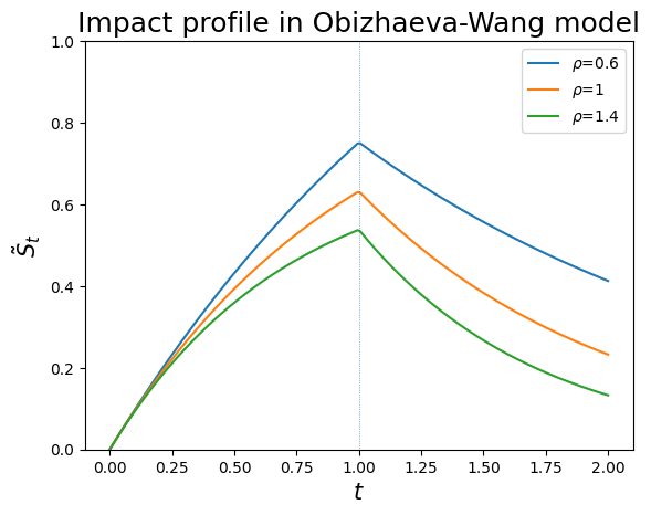

Optimal strategy in Obizhaeva-Wang

The Euler-Lagrange equation in this case reads:

\[ \eta \int_t^T\,v_s\,e^{-\rho\,(s-t)}\,\mathrm{d}s + \eta \int_0^t\,v_s\,e^{-\rho\,(t-s)}\,\mathrm{d}s = \lambda. \]

which may be rewritten as

\[\int_0^T\,v_s\,e^{-\rho\,|t-s|}\,\mathrm{d}s = \frac\lambda\eta\]

which is a Fredholm integral equation of the first kind.

The solution is

\[v_t = \frac\lambda\eta \,\left\{\delta(t)+\rho+\delta(T-t)\right\}\]

The Lagrange multiplier $\lambda$ is determined by

\[-X = x_T - x_0 = \int_0^T\, v_t \,\mathrm{d}t = \frac\lambda\eta \, \left(2+\rho\,T\right)\]

Thus, $\displaystyle \frac\lambda\eta = -\frac X{2 + \rho T}$ and

\[ v_t = -\frac X{2 + \rho T}\left\{\delta(t)+\rho+\delta(T-t)\right\}. \]

The optimal strategy consists of block trades at $t=0$ and $t=T$ and continuous trading at the constant rate $\rho$ between these two times.

Note

The case $\rho = 0$ corresponds to the Almgren-Chriss model with only permanent impact. In this case, the strategy suggests a block trade of half of the total shares at the beginning and a block trade of the other in the end. In fact, in this case all strategies are optimal since the expected cost is a constant, independent of the strategies!

Obizhaeva-Wang as a control problem

We may recast the optimal execution problem in the Obizhaeva-Wang model as a control problem as follows.

Let

\[ Y_t = \eta \int_0^t e^{-\rho(t-s)} v_s \mathrm{d}s. \]

Thus, we can rewrite the dynamic for $S_t$ as $S_t = s_0 + Y_t + \sigma_S Z_t$. It follows that the state equations are given by

\[\begin{align*} & \mathrm{d}X_t = v_t \mathrm{d}t, \quad X_0 = X \\ & \mathrm{d}Y_t = \left\{\eta v_t - \rho Y_t \right\}\mathrm{d}t, \quad Y_0 = 0 \\ \end{align*}\]

Objective functional (the expected cost)

\[\begin{align*} & \int_0^T y_t v_t \mathrm{d}t. \end{align*}\]

Notice that we end up with a deterministic control problem.

Value function

As always, the value function $J$ is defined as

\[ J(t, x, y) = \min_v \int_t^T y_s v_s \mathrm{d}s. \]

HJB equation

The value function will satisfy the following HJB equation.

\[\begin{align*} & J_t + \min_v\{yv + v J_x + (\eta v - \rho y)J_y \} \\ &= J_t - \rho y J_y + \min_v\{(y + J_x + \eta J_y) v\} \\ &= 0 \end{align*}\]

Turns out the control theory formulation of the optimal execution problem under Obizhaeva-Wang model is pretty tricky since

\[ \min_v\{(y + J_x + \eta J_y) v\} = \left\{\begin{array}{ll} - \infty & \text{if } y + J_x + \eta J_y \neq 0, \\ 0 & \text{if } y + J_x + \eta J_y = 0. \end{array}\right. \]

Special treatment for this type of problems are required.

注: HJB 方程, 全称 Hamilton–Jacobi–Bellman Equation. 简单来说: HJB 方程是动态规划在连续时间中的表达形式, 是最优化控制问题的中心工具. 其解就是所谓的 value function, 代表「在给定状态和时间点, 从现在开始最优执行能确保的最低 (或最大) 代价/收益」.

一般说来, 我们定义 value function, 得到对应的 HJB 方程, 然后求解 HJB 方程, 得到 value function 的表达式.

Combining Almgren-Chriss and Obizhaeva-Wang: the ACOW model

We add up the Almgren-Chriss model and the Obizhaeva-Wang model as

\[\begin{align*} & S_t = s_0 + \gamma (X_t - X_0) + Y_t + \sigma_S W_t, \\ & \tS_t = S_t + \eta v_t, \end{align*}\]

where

\[ Y_t = \int_0^t e^{-\rho(t - s)} \phi v_s \mathrm{d}s + \sigma \int_0^t e^{-\rho(t-s)} \mathrm{d}Z_s \]

be the price impact (due to trading). Then $Y_t$ satisfies the ODE

\[ \mathrm{d} Y_t = \{\phi v_t - \rho Y_t\}\mathrm{d}t + \sigma \mathrm{d}Z_t, \quad Y_0 = 0. \]

$S_t$: efficient/mid price
$\tilde S_t$: traded price
$Y_t$: (stochastic) impact to the efficient/mid price due to trading as in Obizhaeva-Wang
$\phi v_t$: linear instantaneous impact
$\eta v_t$: linear temporary impact
$\gamma (X_t - X_0)$: linear permanent impact

Note

Without the $Y$ term, the model reduces to Almgren-Chriss.
If $\gamma = \eta = \sigma = 0$, the model reduces to Obizhaeva-Wang.
The rationale is that Almgren-Chriss takes care of the permanent impact component whereas the trasient impact component for Obizhaeva-Wang.

Impact profile under the model

import numpy as np
import matplotlib.pyplot as plt
import scipy.stats as ss

T = 1
twap_AC = lambda t: t/T*(t <= T) + T*(t > T)
rho = 1.5
m = 2/3
def twap_model(t):
    term1 = (1 - np.exp(-rho*t))*(t <= T) 
    term2 = (1 - np.exp(-rho*T))*np.exp(rho*(T-t))*(t > T) 
    invent = m*(term1 + term2)/rho
    return invent + twap_AC(t)

t = np.linspace(0, 2, 200)
#plt.figure(figsize=(8, 6))
plt.plot(t, twap_AC(t), ls='dotted', color='blue', label='Almgren-Chriss')
plt.plot(t, twap_model(t), ls='dashed', color='blue', label='ACOW')
plt.vlines(x=1, ymin=0, ymax=2, linewidth=0.5, ls='dotted')
plt.ylim([0, 1.8])
plt.xlabel(r'$t$', fontsize=15)
plt.ylabel(r'$\tilde S_t$', fontsize=15)
plt.title('Impact profile under TWAP', fontsize=18)
plt.legend();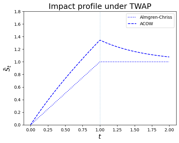

Control problem

State equations

\[\begin{align*} & \mathrm{d}X_t = v_t \mathrm{d}t, \quad X_0 = X \\ & \mathrm{d}Y_t = \left\{\phi v_t - \rho Y_t \right\}\mathrm{d}t + \sigma \mathrm{d}Z_t, \quad Y_0 = 0, \\ & S_t = s_0 + \gamma (X_t - X_0) + Y_t + \sigma_S W_t \\ & s_0 - \tS_t = -\gamma (X_t - X_0) - Y_t - \sigma_S W_t - \eta v_t \end{align*}\]

Objective functional (the expected P&L, marked to the price $s_0$)

\[\begin{align*} & \Eof{X_T(S_T - s_0) + \int_0^T (s_0 - \tS_t) \mathrm{d}X_t} \\ &= \Eof{X_T \{\gamma (X_T - X_0) + Y_T + \sigma_S W_T\} - \int_0^T \left\{\gamma (X_t - X_0) + Y_t + \sigma_S W_t + \eta v_t \right\} \mathrm{d}X_t} \end{align*}\]

Note that, by applying integration by parts, we have

\[\begin{align*} & -\gamma \int_0^T (X_t - X_0) \mathrm{d}X_t -\int_0^T (Y_t + \sigma_S W_t) \mathrm{d}X_t - \eta \int_0^T v_t^2 \mathrm{d}t \\ &= -\frac\gamma2 (X_T - X_0)^2 - X_T (Y_T + \sigma_S W_T) + X_0 (Y_0 + \sigma_S W_0) + \int_0^T X_t \mathrm{d}Y_t + \sigma_S \int_0^T X_t \mathrm{d}W_t - \eta \int_0^T v_t^2 \mathrm{d}t \\ &= -\frac\gamma2 (X_T - X_0)^2 -X_T (Y_T + \sigma_S W_T) + \int_0^T X_t \left\{\phi v_t - \rho Y_t \right\} \mathrm{d}t + \sigma \int_0^T X_t \mathrm{d}Z_t + \sigma_S \int_0^T X_t \mathrm{d}W_t - \eta \int_0^T v_t^2 \mathrm{d}t \end{align*}\]

Thus,

\[\begin{align*} & \Eof{X_T \{\gamma (X_T - X_0) + Y_T + \sigma_S W_T)\} - \int_0^T \{\gamma (X_t - X_0) + Y_t + \sigma_S W_t + \eta v_t\} v_t \mathrm{d}t} \\ &= \Eof{ \frac\gamma2 (X_T^2 + X_0^2) + \int_0^T X_t \left\{\phi v_t - \rho Y_t \right\} - \eta v_t^2 \mathrm{d}t} \end{align*}\]

Penalize the final block trade by $-\beta X_T^2$. The objective functional reads

\[\begin{align*} &= \frac\gamma2 X_0^2 + \Eof{\left(\frac\gamma2 - \beta\right) X_T^2 + \phi \int_0^T X_s dX_s - \int_0^T \left(\rho X_s Y_s + \eta v_s^2\right) \mathrm{d}s} \\ &= \frac{\gamma - \phi}2 X_0^2 + \Eof{\left(\frac{\gamma + \phi}2 -\beta\right) X_T^2 - \int_0^T \left(\rho X_s Y_s + \eta v_s^2\right) \mathrm{d}s}. \end{align*}\]

Matrix notations

Rewrite the equation in matrix notations.

\[\begin{align*} & \bX = \left[\begin{array}{c} x \\ y \end{array}\right], \\ & \mbP = \left[\begin{array}{cc} \frac{\gamma + \phi}2 - \beta & 0 \\ 0 & 0 \end{array}\right], \qquad \mbQ = \left[\begin{array}{cc} 0 & -\frac\rho2 \\ -\frac\rho2 & 0 \end{array}\right], \qquad \mbS = \left[0 \quad 0\right], \qquad \mbR = -\eta, \\ & \mbA = \left[\begin{array}{cc} 0 & 0 \\ 0 & -\rho \end{array}\right], \qquad \mbB = \left[\begin{array}{c} 1 \\ \phi \end{array}\right], \qquad \bSigma = \left[\begin{array}{c} 0 \\ \sigma \end{array}\right]. \end{align*}\]

LQ problem

We obtain the following LQ control problem

\[ \max_u \Eof{\bX_T' \mbP \bX_T + \int_0^T \left(\bX_t' \mbQ \bX_t + \bu_t' \mbR \bu_t \right) \mathrm{d}t}, \]

with the controlled SDE given by

\[ \mathrm{d}\bX_t = (A \bX_t + \mbB v_t)\mathrm{d}t + \bSigma \mathrm{d}Z_t \]

注: LQ (Linear Quadratic) control problem: 线性二次型控制问题, 是一种特殊的最优控制问题, 其目标是最小化一个二次型的代价函数, 同时满足线性动态系统的约束条件.

Value function and HJB equation

Let $V$ be the value function

\[ V(t, \bx) = \max_{\bu} \Eof{\left. \bX_T' \mbP \bX_T + \int_t^T \left(\bX_s' \mbQ \bX_s + \bu_s' \mbR \bu_s \right) \mathrm{d}s\right|\bX_t = \bx}. \]

$V$ satisfies the following HJB equation

\[ V_t + \frac12\tr(\bSigma\bSigma'\nabla^2 V) + \max_{\bu}\left\{(\mbA \bx + \mbB \bu)' \nabla V + \bx'\mbQ\bx + \bu_t' \mbR \bu_t \right\} = 0 \]

with terminal condition $V(T, \bx) = \bx'\mbP\bx$.

Note

$\mbR = -\eta$ is negative definite since we have a maximization problem.

Optimal control

\[ \bu = - \frac12 \mbR^{-1} \mbB'\nabla V. \]

\[\begin{align*} & V_t + \frac12\tr(\bSigma\bSigma'\nabla^2 V) + \max_{\bu}\left\{(\mbA \bx + \mbB \bu)' \nabla V + \bx'\mbQ\bx + \bu'\mbR\bu \right\} \\ &= V_t + \frac12\tr(\bSigma\bSigma'\nabla^2 V) + \bx'\mbA' \nabla V + \bx'\mbQ\bx - \frac14 \nabla V' \mbB \mbR^{-1} \mbB' \nabla V \end{align*}\]

Ansatz

Assume the ansatz for value function $V(t, \bx) = \bx' H_1 \bx + H_0$.

The optimal (feedback) control $\bu^*$ becomes

\[ \bu^* = - \frac12 \mbR^{-1} \mbB'\nabla V = \frac1{\eta} \mbB' H_1 \bx \]

Matrix Riccati equation

Compare the coefficients and obtain the matrix Riccati equation

\[\begin{align*} & \dot H_1 - H_1\mbB\mbR^{-1}\mbB'H_1 + \mbA' H_1 + H_1 \mbA + \mbQ = 0 \\ & \dot H_0 + \tr(\bSigma\bSigma'H_1) = 0 \end{align*}\]

with terminal condition $H_1(T) = \mbP$ and $H_0(T) = 0$.

\[\begin{align*} & \dot H_1 + \frac1\eta H_1\mbB\mbB'H_1 + \mbA' H_1 + H_1 \mbA + \mbQ = 0 \\ & \dot H_0 + \tr(\bSigma\bSigma'H_1) = 0 \end{align*}\]

注: 黎卡提方程 (Riccati Equation) 是一类非线性一阶常微分方程, 广泛应用于控制理论、量子力学、金融数学等多个领域. Ricatti 方程通常表示为: \[ \frac{\mathrm{d} y}{\mathrm{d} x} = P(x)y^2 + Q(x)y + R(x), \] 其中 $P(x)$, $Q(x)$, $R(x)$ 是已知的函数, $y(x)$ 是未知函数.

在最优控制问题中, 黎卡提方程用于求解代数黎卡提方程 (ARE, Algebraic Riccati Equation) 或微分黎卡提方程 (DRE, Differential Riccati Equation).

代数黎卡提方程 (ARE) 是一种特殊的黎卡提方程, 其形式为: \[ 0 = A'X + XA - XBR^{-1}B'X + Q, \] 其中 $A$, $B$, $Q$, $R$ 是已知矩阵, $X$ 是未知矩阵. ARE 在最优控制问题中用于无限时间的最优控制问题.
微分黎卡提方程 (DRE) 是一种时间相关的黎卡提方程, 其形式为: \[ \dot X = A'X + XA - XBR^{-1}B'X + Q, \] 其中 $\dot X$ 是 $X$ 关于时间的导数. DRE 在最优控制问题中用于有限时间的最优控制问题.

Solution to the Riccati equation

The solution to the matrix Riccati equation for $H_1$ can be characterized by the solution to the following linear system of equations

\[ H_1 = M N^{-1}, \]

where $M$, $N$ satisfy the linear ODEs

\[ \frac{\mathrm{d}}{\mathrm{d}t} \left[\begin{array}{c} M \\ N \end{array}\right] = \left[\begin{array}{cc} -\mbA & -\mbQ \\ \frac1{\eta}\mbB \mbB' & \mbA \end{array}\right] \, \left[\begin{array}{c} M \\ N \end{array}\right] \]

with terminal conditions $M_T = H_1(T) = \mbP$ and $N_T = I$.

The solution to the linear system can be written as

\[ \left[\begin{array}{c} M \\ N\end{array}\right] =e^{-(T-t)\Psi} \, \left[\begin{array}{c} \mbP \\ I \end{array}\right] \]

where

\[ \Psi = \left[\begin{array}{cc} -\mbA & -\mbQ \\ \frac1{\eta}\mbB \mbB' & \mbA \end{array}\right] \, \left[\begin{array}{c} M \\ N \end{array}\right] \]

The expected trading trajectory $x_t = \Eof{X_t}$ under optimal control $\bu^*$ satisfies

\[\begin{align*} & \dot x_t = \frac1{\eta} \mbB' H_1 \bx, \\ & \dot y_t = \frac\phi{\eta} \mbB' H_1 \bx - \rho y_t, \end{align*}\]

where $y_t = \Eof{Y_t}$.

Note that we have

\[ \phi \dot x_t - (\dot y_t + \rho y_t) = 0 \]

Thus,

\[ e^{\rho t} y_t - y_0 = \phi (x_t - x_0) \quad \Longrightarrow \quad y_t = e^{-\rho t}y_0 + e^{-\rho t}\phi(x_t - x_0) = e^{-\rho t}\phi(x_t - x_0) \]

since $y_0 = 0$.

Numerical examples

from scipy.linalg import expm
from scipy.integrate import odeint

# liquidation horizon
T = 1

# number of shares to liquidate
x0 = 20_000

# mean reverting rate rho
# rho in the exponential decay kernel
rho = 10 # 1e-3

# parameters for market impact from Almgren-Chriss
eta = 2.5*1e-6 # temporary impact coefficient
gamma = 2.5*1e-7 # permanent impact coefficient

# final block trade penalty
beta = 1000*eta #, 100*eta, 1000*eta, 10_000*eta

# coefficient for inventory cost
# coefficient for linear instantaneous impact function
phi = 50*eta # eta, 5*eta, 10*eta, 100*eta

print(f'(gamma + phi)/2 - beta is {(gamma+phi)/2 - beta}.')

(gamma + phi)/2 - beta is -0.0024373749999999994.

# matrices
A = np.array([0, 0, 0, -rho]).reshape(2, 2)
P = np.array([(gamma + phi)/2 - beta, 0, 0, 0]).reshape(2, 2)
Q = np.array([0, -rho/2, -rho/2, 0]).reshape(2, 2)
B = np.array([1, phi]).reshape(2, 1)

# Psi
Psi = np.array([[0, 0, 0, rho/2], [0, rho, rho/2, 0], [1/eta, phi/eta, 0, 0], 
                [phi/eta, phi**2/eta, 0, -rho]])

# solution H1
def H1(t):
    # Matrix [P I]'
    PI = np.concatenate([P.reshape(4), np.identity(2).reshape(4)]).reshape(4, 2)
    # exponential Psi times [P I]'
    ePsiPI = lambda t: expm(-(T-t)*Psi).dot(PI)    
    M, N = ePsiPI(t)[:2], ePsiPI(t)[2:]
    return M.dot(np.linalg.inv(N))

# first order criterion for v
def v_opt(bx, t):
    BtH = B.transpose().dot(H1(t))
    return BtH.dot(bx)/eta

# ODE for x and y
def f(bx, t):
    x = bx[0]
    y = bx[1]
    dx = v_opt(bx, t)
    dy = phi*v_opt(bx, t) - rho*y
    return np.array([dx, dy]).reshape(2)

# solve optimal x and y numerically
def solve_opt_xy(n_steps=500): 
    t = np.linspace(0, T, n_steps+1)
    bx0 = np.array([x0, 0])
    soln1 = odeint(f, bx0, t)
    x_opt = soln1[:, 0]
    y_opt = soln1[:, 1]
    return x_opt, y_opt

n_steps = 200
t = np.linspace(0, 1, n_steps+1)
x, y = solve_opt_xy(n_steps)

# plot optimal trajectory for x
#plt.figure(figsize=(8, 6))
plt.plot(t, x)
plt.xlabel(r'$t$', fontsize=15)
plt.ylabel(r'$x$', fontsize=15)
plt.hlines(y=0, xmin=0, xmax=1, ls='dotted');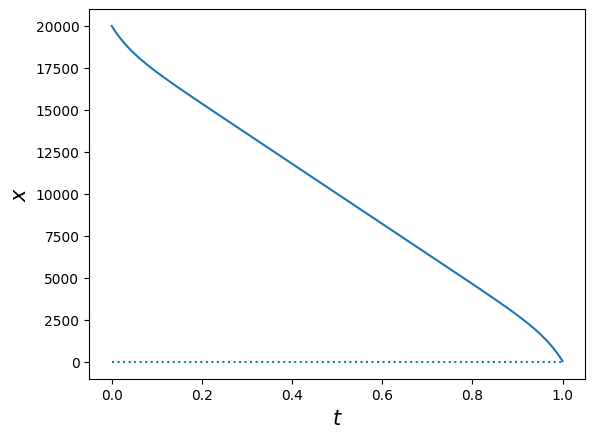

# plot trajectory for y under optimal policy
#plt.figure(figsize=(8, 6))
plt.plot(t, y)
plt.xlabel(r'$t$', fontsize=15)
plt.ylabel(r'$y$', fontsize=15)
plt.hlines(y=0, xmin=0, xmax=1, ls='dotted', color='k');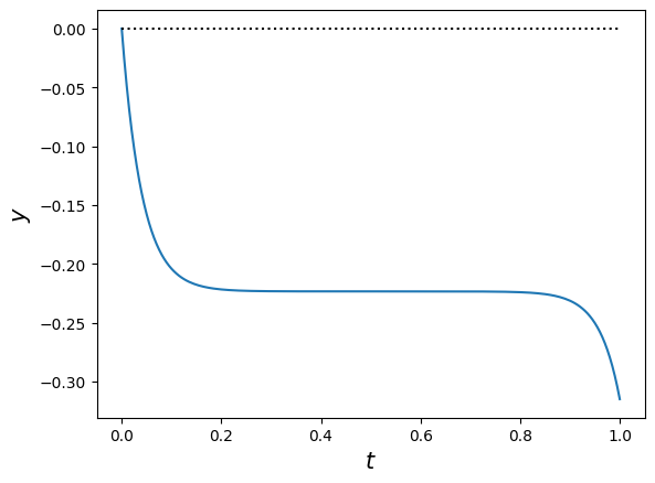

# the optimal trading rate v
v =np.array([])
for i in range(len(t)):
    BtH = B.transpose().dot(H1(t[i]))
    v = np.concatenate([v, BtH.dot([x[i], y[i]])/eta])

# plot optimal trajectory for v
#plt.figure(figsize=(8, 6))
plt.plot(t, v)
plt.xlabel(r'$t$', fontsize=15)
plt.ylabel(r'$v$', fontsize=15);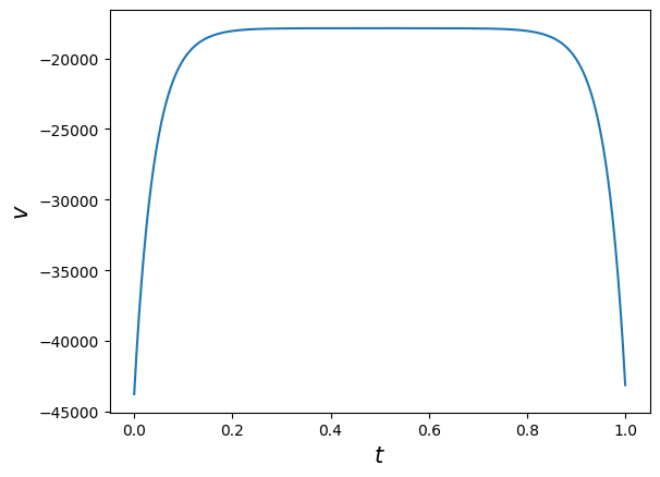

# in fact, v = dx/dt
plt.plot(t[1:], np.diff(x)/np.diff(t));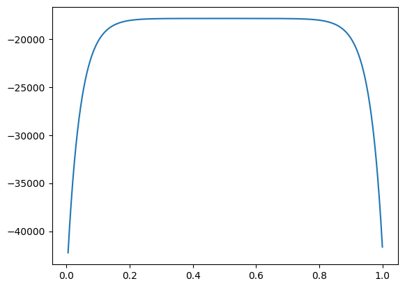

Value distribution

Let’s compare the performance of optimal trading strategy to TWAP and Almgren-Chriss in this setting.

Create a `python` class for evaluating value function by simulation

import numpy as np
from scipy.stats import norm 
import seaborn as sns

class ValueDistribution:
    '''
    x0: number of shares to liquidate/acquire
    T: liquidation/acquistion horizon
    gamma: permanent impact coefficient
    eta: temporary impact coefficient
    rho: mean reverting rate
    beta: final block trade penalty
    phi: transient impact coefficient
    sigma: volatility of transient impact
    '''
    
    def __init__(self, params, strategy, n_steps=100):
        self.T = params['T']
        self.x0 = params['x0']
        self.eta = params['eta']
        self.gamma = params['gamma']
        self.beta = params['beta']
        self.phi = params['phi']
        self.rho = params['rho']
        self.sigma = params['sigma']
        self.n_steps = n_steps
        
        # strategy v as a function of x, y, t
        self.strategy = strategy
        
#        self.alpha = 2*self.eta/(2*self.beta - self.gamma)
        
    def simulate(self, n_sim=10_000):
        n_steps = self.n_steps
        v = self.strategy
        dt = self.T/self.n_steps
        gamma, phi, eta, beta, rho = self.gamma, self.phi, self.eta, self.beta, self.rho
        
        # initialize 
        y = np.zeros([n_sim, n_steps+1])
        x = np.ones([n_sim, n_steps+1])*self.x0
        V0 = np.zeros([n_sim, n_steps+1])

        for step in range(self.n_steps):
            dz = norm.rvs(size=n_sim)*np.sqrt(dt)
            dy = (phi*v(x[:,step], y[:,step], step*dt) - rho*y[:,step])*dt + sigma*dz
            dx = v(x[:,step], y[:,step], step*dt)*dt 
            dV0 = -(rho*x[:,step]*y[:,step] + eta*v(x[:,step], y[:,step], step*dt)**2)*dt
            x[:,step+1] = x[:,step] + dx
            y[:,step+1] = y[:,step] + dy
            V0[:,step+1] = V0[:,step] + dV0

        self.x, self.y, self.V0 = x, y, V0
        self.V = ((gamma + phi)/2 - beta)*x[:,-1]**2 + V0[:,-1]
        return self.V.mean()
    
    def V_hist(self, bins=50, kde=True, stat='density', element='step'):
        sns.histplot(self.V, bins=bins, kde=kde, stat=stat, element=element)
        plt.title('Histogram of V', fontsize=20);
        return None
    
    def __call__(self):
        pass

Policy 1: TWAP

# parameters
sigma = 0.1
params = {'T': T, 'x0': x0, 'eta': eta, 'gamma': gamma, 'rho': rho, 'beta': beta, 'phi': phi, 'sigma':sigma}

# A version of TWAP strategy
alpha = 2*eta/(2*beta - gamma)
v_twap = lambda x, y, t: -x/(T - t + alpha)

# instantiate the class and simulate
vd_twap = ValueDistribution(params=params, strategy=v_twap, n_steps=n_steps)
vd_twap.simulate()

19608.269295580816

Sample path of running reward

n_sim, n_steps = 10_000, 200
dt = T/n_steps
t = np.arange(0, T+dt, dt)
n_path = np.random.choice(n_sim)
plt.plot(t, vd_twap.V0[n_path,:]);
print(n_path)

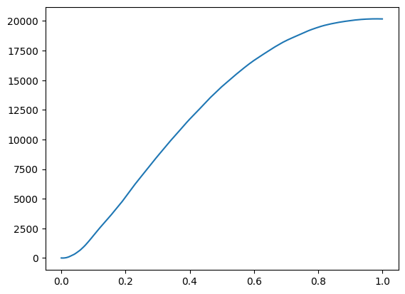
vd_twap.V_hist()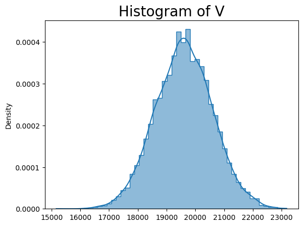

Optimal policy

def v_opt(x, y, t):
    bx = np.column_stack([x, y])
    HB = H1(t).dot(B)
    return bx.dot(HB).flatten()/eta

vd_opt = ValueDistribution(params=params, strategy=v_opt, n_steps=n_steps)
vd_opt.simulate()

19744.088225206633

vd_opt.V_hist()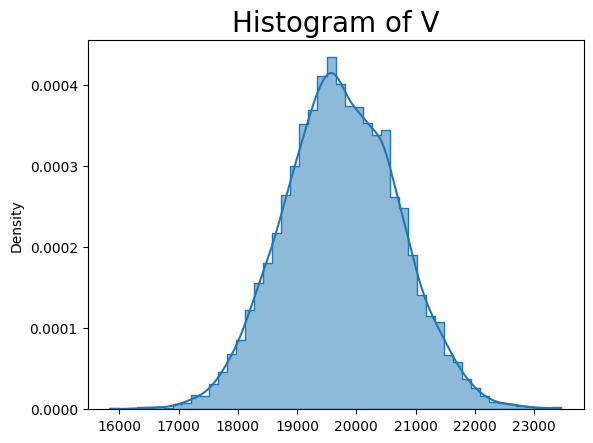

Put together the histograms

sns.histplot(vd_twap.V, bins=50, stat='density', element='step', kde=True);
sns.histplot(vd_opt.V, bins=50, stat='density', color='orange', element='step', kde=True);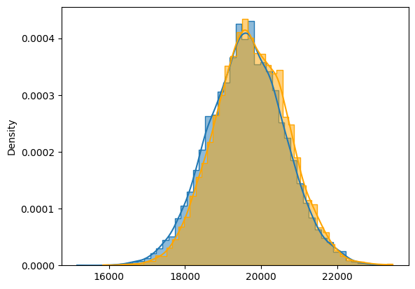

Sample path of liquidation

n_path = np.random.choice(n_sim)
plt.plot(t, vd_opt.x[n_path,:])
plt.plot(t, vd_twap.x[n_path,:], color='orange');
n_path

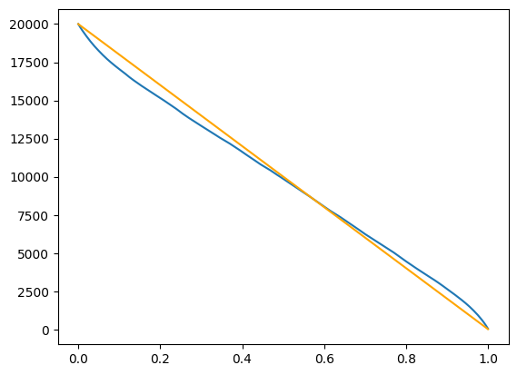
Sample path of transient impact

#plt.figure(figsize=(12,6))
plt.subplot(1, 2, 1)
plt.plot(t, vd_opt.y[n_path,:])
plt.title('Transient impact under optimal strategy', fontsize=15)
plt.subplot(1, 2, 2)
plt.title('Transient impact under TWAP', fontsize=15)
plt.plot(t, vd_twap.y[n_path,:]);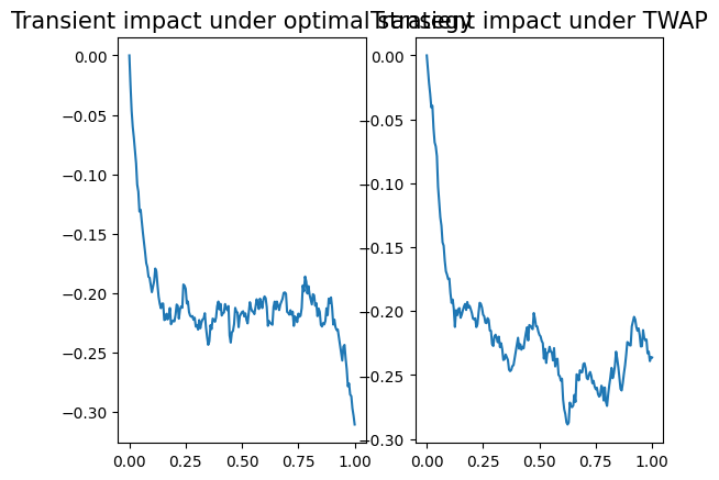

References

Robert Almgren and Neil Chriss, Optimal execution of portfolio transactions, Journal of Risk, 3, 5–40, (2001).
Emanuel Bacry, Adrian Iuga, Matthieu Lasnier, and Charles-Albert Lehalle, Market impacts and the life cycle of investors orders, Market Microstructure and Liquidity, 1(2), 1550009, (2015).
Jim Gatheral, Lecture notes on market microstructure models, Baruch MFE course .
Anna Obizhaeva and Jiang Wang, Optimal trading strategy and supply/demand dynamics, Journal of Financial Markets, 16(1), 1–32, (2013).
Elia Zarinelli, Michele Treccani, J. Doyne Farmer, and Fabrizio Lillo, Beyond the square root: Evidence for logarithmic dependence of market impact on size and participation rate, Market Microstructure and Liquidity, 1(2), 1550004, (2015).

A Simple Lecture Notes

概述
- 主题: 价格冲击 (market impact) 及最优执行 (optimal execution)
- 核心问题: 大额交易 (metaorder) 如何影响市场价格? 如何在承受冲击成本和价格风险之间取得平衡, 以实现最优交易执行?
核心术语
- Metaorder (元订单): 体量足够大, 需拆分执行的订单.
- 子订单 (child order): 元订单的拆分单元.
- Impact profile (冲击剖面): 元订单执行期间及执行后, 平均价格随时间的轨迹.
- Completion (完成): 最后一笔子订单成交的时刻.
- Spread cost (点差成本): 买入/卖出时吃掉的半个买卖价差.
元订单的市场冲击
1. 定性描述
- 买盘倾向推高价格, 卖盘倾向压低价格。
- 市场冲击可分为瞬时冲击 (temporary impact) 和永久冲击 (permanent impact).
1. 平方根法则 (Square‐Root Impact Law)
- 经验公式: \[ \Delta P \approx \text{Spread cost} + \alpha \cdot \sigma \cdot \sqrt{\frac{Q}{V}}, \] 其中
  - $\sigma$: 日内美元波动率
  - $V$: 日均成交量
  - $Q$: 元订单体量
  - $\alpha$: 冲击系数 (impact coefficient)
常见执行算法
- TWAP (Time-Weighted Average Price): 等速切分、等间隔执行
- VWAP (Volume-Weighted Average Price): 按市场成交量比例参与交易
- POV (Percentage-of-Volume): 固定日内市场成交量百分比
- IS (Implementation Shortfall): 前期快速执行、后期放缓, 以平衡滑点成本与市场风险
Almgren–Chriss 模型
1. 模型设定
- 资产价格:
  \[ S_t = S_0 + \gamma (X_t - X_0) + \sigma_S W_t, \] 其中 $v_s$ 为交易速率，$\eta$ 为冲击系数
- 成本函数:
  \[ C_T(x) = \int_0^T \left( \gamma v_t^2 + \eta v_t^2 \right) \mathrm{d}t + \int_0^T (S_0 - S_t) \mathrm{d}x_t, \] $\lambda$: 风险厌恶系数
1. 最优策略
- 风险中性 ($\lambda = 0$): 最优执行为等速执行 (TWAP)
- 风险厌恶($\lambda > 0$): 求解二阶常微分方程, 得到渐进收敛于均匀速率的交易轨迹
1. 优缺点
- 易于分析与实现, 成为算法交易基础
  – 冲击无回落, 与实证的瞬时衰减不符
  – 永久冲击线性假设与平方根规律不一致
Obizhaeva–Wang 模型
1. 模型设定
- 冲击脉冲响应 (exponential decay):
  \[ S_t = S_0 + \eta \int_0^t v_s e^{-\rho(t-s)} \mathrm{d}s + \sigma_S Z_t, \] 其中 $\rho$ 为衰减速率
1. 特点
- 冲击线性、衰减符合指数律
- 更符合高频撮合市场微结构
ACOW 模型 (Almgren–Chriss + Obizhaeva–Wang)
- 结合永久冲击 (AC) 和瞬时指数衰减冲击 (OW)
- 状态方程 + 最优控制问题
- 可调节参数 $\gamma, \eta, \sigma$ 控制永久与瞬时冲击
小结与讨论
- 市场冲击研究的目的:
  - 量化大额交易对价格的影响
  - 在成本与风险之间做出量化权衡
- 未来方向:
  - 非线性冲击函数、非高斯噪声
  - 多资产组合清算
  - 深度学习与在线自适应执行算法

References

Almgren, Robert, and Neil Chriss. 2001. “Optimal Execution of Portfolio Transactions.” Journal of Risk 3 (2): 5–39. https://doi.org/10.21314/JOR.2001.041.

Bacry, Emmanuel, Adrian Iuga, Matthieu Lasnier, and Charles-Albert Lehalle. 2014. “Market Impacts and the Life Cycle of Investors Orders.” https://arxiv.org/abs/1412.0217.

Obizhaeva, Anna A., and Jiang Wang. 2013. “Optimal Trading Strategy and Supply/Demand Dynamics.” Journal of Financial Markets 16 (1): 1–32. https://doi.org/10.1016/j.finmar.2012.09.001.

Zarinelli, Elia, Michele Treccani, J. Doyne Farmer, and Fabrizio Lillo. 2014. “Beyond the Square Root: Evidence for Logarithmic Dependence of Market Impact on Size and Participation Rate.” https://arxiv.org/abs/1412.2152.

Lecture 6: Optimal execution under price impact

Agenda

What is market or price impact?

The square-root formula for market impact

Commonly applied algorithms

Terminology

Schematic of impact profile

Stylized features of impact profile

Empirical market impact profiles from (Bacry et al. 2014)

Empirical market impact profiles from (Zarinelli et al. 2014)

Notations

Almgren and Chriss

The price impact model of Almgren and Chriss

Note

Impact profile in the Almgren and Chriss model

Inconsistency with empirical observation

P&L and cost of trading of a trading strategy

Implementation shortfall as cost of trading

P&L in Almgren-Chriss model

Expected cost of TWAP in the Almgren and Chriss model

Optimal strategy of a risk neutral trader

Variational problem

Risk neutral trader: TWAP is optimal in Almgren-Chriss

Penalty by quadratic variation

Mean-QV trader: The Almgren-Chriss strategy

Note

Applications of the Almgren-Chriss framework

Summary on the Almgren-Chriss model

Transient impact models

Note

P&L and cost of trading in transient impact model

The optimal strategy of a risk neutral trader

Lagrange multiplier

Euler-Lagrange equation

The Obizhaeva and Wang model

Impact profile in the Obizhaeva and Wang model

Optimal strategy in Obizhaeva-Wang

Note

Obizhaeva-Wang as a control problem

Value function

HJB equation

Combining Almgren-Chriss and Obizhaeva-Wang: the ACOW model

Note

Impact profile under the model

Control problem

Matrix notations

LQ problem

Value function and HJB equation

Note

Optimal control

Ansatz

Matrix Riccati equation

Solution to the Riccati equation

Numerical examples

Value distribution

Create a python class for evaluating value function by simulation

Policy 1: TWAP

Sample path of running reward

Optimal policy

Put together the histograms

Sample path of liquidation

Sample path of transient impact

References

A Simple Lecture Notes

References

Create a `python` class for evaluating value function by simulation