Topics in Quantitative Finance, Summer 2025

Lecture 3: The Black-Merton-Scholes model and beyond I

Tai-Ho Wang (王太和)

\[ \newcommand{\bea}{\begin{eqnarray}} \newcommand{\eea}{\end{eqnarray}} \newcommand{\supp}{\mathrm{supp}} \newcommand{\cA}{\mathcal{A} } \newcommand{\F}{\mathcal{F} } \newcommand{\cF}{\mathcal{F} } \newcommand{\E}{\mathbb{E} } \newcommand{\Eof}[1]{\mathbb{E}\left[ #1 \right]} \newcommand{\Etof}[1]{\mathbb{E}_t\left[ #1 \right]} \newcommand{\Sdof}[1]{\mathbb{Sd}\left[ #1 \right]} \def\Cov{{ \mbox{Cov} }} \def\Var{{ \text{Var} }} \newcommand{\1}{\mathbf{1} } \newcommand{\p}{\partial} \newcommand{\PP}{\mathbb{P} } \newcommand{\Pof}[1]{\mathbb{P}\left[ #1 \right]} \newcommand{\QQ}{\mathbb{Q} } \newcommand{\R}{\mathbb{R} } \newcommand{\DD}{\mathbb{D} } \newcommand{\HH}{\mathbb{H} } \newcommand{\spn}{\mathrm{span} } \newcommand{\cov}{\mathrm{cov} } \newcommand{\HS}{\mathcal{L}_{\mathrm{HS}} } \newcommand{\Hess}{\mathrm{Hess} } \newcommand{\trace}{\mathrm{trace} } \newcommand{\LL}{\mathcal{L} } \newcommand{\s}{\mathcal{S} } \newcommand{\ee}{\mathcal{E} } \newcommand{\ff}{\mathcal{F} } \newcommand{\hh}{\mathcal{H} } \newcommand{\bb}{\mathcal{B} } \newcommand{\dd}{\mathcal{D} } \newcommand{\g}{\mathcal{G} } \newcommand{\half}{\frac{1}{2} } \newcommand{\T}{\mathcal{T} } \newcommand{\bit}{\begin{itemize}} \newcommand{\eit}{\end{itemize}} \newcommand{\beq}{\begin{equation}} \newcommand{\eeq}{\end{equation}} \newcommand{\tr}{\mbox{tr}} \newcommand{\inn}[2]{\left\langle #1, #2 \right\rangle} \newcommand{\bX}{\boldsymbol X} \newcommand{\bm}{\boldsymbol m} \newcommand{\bx}{\boldsymbol x} \newcommand{\by}{\boldsymbol y} \newcommand{\bmu}{\boldsymbol\mu} \newcommand{\bxi}{\boldsymbol\xi} \]

Agenda

Black-Merton-Scholes model
Black-Merton-Scholes formula for call and put options
Greeks
Subtlety in self-financing
Delta and delta-gamma hedges
Dynamic hedging
Deep hedging

Remark

Black-Merton-Scholes 模型是用于期权定价的经典模型
Call option: 看涨期权; Put option: 看跌期权
Greeks 是衡量期权价格对市场变量变化敏感度的指标
自融资策略(self-financing)是指在不注入额外资金的情况下进行投资组合调整.
hedging 是指通过对冲策略来降低风险. 对冲指通过调整标的资产的数量, 使得投资组合的价值对市场变量的变化不敏感.
1. Delta 对冲, 投资组合对标的资产价格的一阶变动免疫
2. Delta-Gamma 对冲, 投资组合对标的资产价格的二阶变动免疫
Dynamic Hedging
1. 动态对冲是指在期权到期前, 根据市场变化不断调整投资组合, 以保持对冲效果.
2. Deep Hedging 是指使用深度学习模型来优化动态对冲策略, 通过学习历史数据中的模式来提高对冲效果.

Black-Merton-Scholes

From the Wikipage:

The Black–Scholes or Black–Scholes–Merton model is a mathematical model for the dynamics of a financial market containing derivative investment instruments. From the partial differential equation in the model, known as the Black–Scholes equation, one can deduce the Black–Scholes formula, which gives a theoretical estimate of the price of European-style options and shows that the option has a unique price regardless of the risk of the security and its expected return (instead of replacing the security’s expected return with the risk-neutral rate). The formula led to a boom in options trading and provided mathematical legitimacy to the activities of the Chicago Board Options Exchange and other options markets around the world. It is widely used, although often with adjustments and corrections, by options market participants.
The key idea behind the model is to hedge the option by buying and selling the underlying asset in just the right way and, as a consequence, to eliminate risk. This type of hedging is called “continuously revised delta hedging” and is the basis of more complicated hedging strategies such as those engaged in by investment banks and hedge funds.
The Black–Scholes formula has only one parameter that cannot be directly observed in the market: the average future volatility of the underlying asset, though it can be found from the price of other options. Since the option value (whether put or call) is increasing in this parameter, it can be inverted to produce a “volatility surface” (implied volatility) that is then used to calibrate other models ((exotic) derivatives), e.g. for OTC derivatives.

The Black-Scholes world

The Black–Scholes model assumes that the market consists of at least one risky asset, usually called the stock, and one riskless asset, usually called the money market, cash, or bond.

Assumptions on the assets:

(riskless rate) The rate of return on the riskless asset is constant and thus called the risk-free interest rate.
(Brownian motion) The instantaneous log return of stock price is a Brownian motion with drift; and we will assume its drift and volatility are constant (if they are time-varying, we can deduce a suitably modified Black–Scholes formula quite simply, as long as the volatility is not random). As a result, the stock price follows a geometric Brownian motion.
The stock does not pay dividend.

Assumptions on the market:

There exists no arbitrage opportunity.
It is possible to borrow and lend any amount, even fractional, of cash at the riskless rate.
It is possible to buy and sell any amount, even fractional, of the stock, including short selling.
Frictionless market: the transactions do not incur any fees or costs.

Black-Scholes model

Assume the price of the underlying asset follows the stochastic differential equation

\[ \frac{\mathrm{d}S_t}{S_t} = \mu \mathrm{d}t + \sigma \mathrm{d}W_t, \]

where

$\mu$: (constant) expected return
$\sigma$: (constant) volatility
$W_t$: standard Brownian motion

For each time $t$, $S_t$ is log-normally distributed. More precisely,

\[ S_t \sim S_0 \exp\left[\left(\mu - \frac{\sigma^2}{2}\right)t + \sigma \sqrt t Z \right] \]

where $Z$ is a standard normal random variable.

Note

$S_t$ has the closed form expression

\[ S_t = S_0 e^{\left(\mu - \frac{\sigma^2}2 \right) t+ \sigma W_t} \]

and is also referred to as a geometric Brownian motion.

The price can never be negative, i.e., $S_t \geq 0$ for all $t \geq 0$.

Pricing under the Black-Scholes model

Assume the price of a call option $C$ is a (smooth enough) function of the calendar time $t$ and the underlying asset $S$. Consider the portfolio $\Pi$ consisting of selling a call option and holding $\Delta$ shares of $S$.

The value of $\Pi$ at time $t$ is \[ \Pi_t = -C(t, S_t) + \Delta S_t \]
Self-financing strategy

\[ \mathrm{d} \Pi_t = -\mathrm{d}C_t + \Delta \mathrm{d}S_t \]

The change of call price is given by

\[\begin{equation} \begin{aligned} \mathrm{d}C(t, S_t) &= C_t \, \mathrm{d}t + C_S \, \mathrm{d}S_t + \frac{1}{2} C_{SS} (\mathrm{d}S_t)^2 \\ &= C_S \sigma S \, \mathrm{d}W_t + \left( C_t + \frac{1}{2} \sigma^2 S^2 C_{SS} + \mu S C_S \right) \mathrm{d}t \end{aligned} \end{equation}\]

Hence the infinitesimal change of $\Pi$ at time $t$ is

\[\begin{equation} \begin{aligned} \mathrm{d} \Pi_t &= -\mathrm{d}C_t + \Delta \, \mathrm{d}S_t \\ &= -\left[ C_t + \frac{1}{2} \sigma^2 S^2 C_{SS} + \mu S (C_S - \Delta) \right] \mathrm{d}t - \sigma S (C_S - \Delta) \, \mathrm{d}W_t \end{aligned} \end{equation}\]

Note

$(\mathrm{d}S_t)^2 = \sigma^2 S_t^2 \mathrm{d}t$

Let $\Delta = C_S$, i.e., hold this amount $C_S(t,S_t)$ of underlying assets in the portfolio $\Pi$. Then the infinitesimal change of $\Pi$ becomes

\[ \displaystyle \mathrm{d}\Pi_t = -\left( C_t + \frac12 \sigma^2 S^2 C_{SS} \right) \mathrm{d}t \]

On the other hand, with this choice of $\Delta$, $\Pi$ is riskless (non-random) hence must be like cash in bank account (Arbitrage Pricing Theory), i.e.,

\[ \mathrm{d}\Pi_t = r \Pi_t \mathrm{d}t = r(-C + \Delta S) \mathrm{d}t = r(-C + C_S S) \mathrm{d}t, \]

where $r$ is the interest rate.

Black-Scholes PDE

We conclude that the price $C$ of a call option satisfies

\[\begin{equation} \begin{aligned} \frac{\partial C}{\partial t} + \frac{\sigma^2}{2} S^2 \frac{\partial^2 C}{\partial S^2} + rS \frac{\partial C}{\partial S} - rC = 0, \quad \text{for } 0 < S < \infty, \quad 0 \leq t < T \end{aligned} \end{equation}\]

with terminal condition

\[ C(T,S) = (S - K)^+ \]

and boundary conditions

\[\begin{equation} \begin{aligned} && C(t, 0) = 0, \\ && C(t, S) \sim S - K e^{-r(T-t)} \quad \text{as } S \to \infty, \\ && \text{or more specifically} \quad \lim_{S \to \infty} \frac{C(t, S)}{S} = 1. \end{aligned} \end{equation}\]

Note

The Black-Scholes pricing PDE does not depend on the drift $\mu$.

$C(T,S) = (S-K)^+$ 表示欧式看涨期权在到期时($t= T$)的支付函数. 若股价高于执行价 $K$, 则价值是差额; 否则归零.

这里的 PDE 是通过 Feynamn-Kac 定理得到的:

\[\begin{align*} \mathrm{d} S_t &= r S_t \mathrm{d} t + \sigma S_t \mathrm{d} W_t \\ C(t,s) &= \Eof{e^{-r(T-t)} (S_T - K)^+ \mid S_t = s} \end{align*}\]

那么 PDE 就是 \[ \frac{\partial C}{\partial t} + r S \frac{\partial C}{\partial S} + \frac{\sigma^2}{2} S^2 \frac{\partial^2 C}{\partial S^2} - r C = 0. \]

Solving Black-Scholes PDE

\[ \frac{\p C}{\p t} + \frac{\sigma^2}{2}S^2\frac{\p C^2}{\p S^2} + rS\frac{\p C}{\p S} - rC = 0 \]

$\tau = T - t$

\[ \frac{\p C}{\p \tau} = \frac{\sigma^2}{2}S^2\frac{\p C^2}{\p S^2} + rS\frac{\p C}{\p S} - rC \]

$\xi = \ln S$

\[ \frac{\p C}{\p \tau} = \frac{\sigma^2}{2}\frac{\p C^2}{\p \xi^2} + \left( r -\frac{\sigma^2}{2} \right) \frac{\p C}{\p \xi} - rC \]

$c(\xi,\tau) = e^{r\tau}C(\xi,\tau)$

\[ \frac{\p c}{\p \tau} = \frac{\sigma^2}{2}\frac{\p c^2}{\p \xi^2} + \left( r -\frac{\sigma^2}{2} \right) \frac{\p c}{\p \xi} \]

$\displaystyle x = \xi + \left( r - \frac{\sigma^2}{2} \right) \tau$

\[ \frac{\p c}{\p \tau} = \frac{\sigma^2}{2} \frac{\p^2 c}{\p x^2} \]

In total, we have done the transformation

\[\begin{equation} \begin{aligned} \tau &= T - t, \\ x &= \ln S + \left( r - \frac{\sigma^2}{2} \right) (T - t), \\ c &= e^{r(T-t)} C. \end{aligned} \end{equation}\]

which transforms Black-Scholes equation into heat equation.

The Black-Scholes formula

For call option

\[ C = S e^{-d\tau} N(d_1) - K e^{-r\tau} N(d_2) \]

where $\tau$ is time to expiry, $N(\cdot)$ denotes the cdf for standard normal, and

\[ d_1 = \frac{\log\left(\frac{Se^{-d\tau}}{Ke^{-r\tau}}\right)}{\sigma\sqrt\tau}+ \frac{\sigma\sqrt\tau}2, \qquad d_2 = d_1 - \sigma \sqrt\tau \]

注:

Term	Economic meaning
$S e^{-d\tau} N(d_1)$	Dividend discounted stock price
$K e^{-r\tau}$	Present value of strike price
$N(d_2)$	The probability of the option expires in the money.

注: in the money = 实值, at the money = 平值, out of the money = 虚值.

in the money = the option is worth exercising at expiry, i.e., $S_T > K$.

The $N(d_1)$ is the factor by which the present value of contingent(有条件的) receipt(收入) of the stock, contingent on exercise, exceeds the current value of the stock.

The $N(d_2)$ is the risk-adjusted probability of exercise.

For put option

\[ P = K e^{-r\tau} N(-d_2) - S e^{-d\tau} N(-d_1). \]

$\tau = T - t$

Note

Put-call parity

\[ C - P = S e^{-d\tau} - K e^{-r\tau}. \]
Financial meaning of $N(d_1)$ and $N(d_2)$

import numpy as np
import matplotlib.pyplot as plt
import pandas as pd
from numpy import exp, log, sqrt
from scipy.stats import norm

norm.rvs(size=10) # generate samples from standard normal 
norm.cdf # cdf of standard normal
norm.pdf # pdf for standard normal
norm.ppf # quantile funciton

<bound method rv_continuous.ppf of <scipy.stats._continuous_distns.norm_gen object at 0x0000020A9875EE10>>

print(norm.cdf(0)) # This is N(0) in our notation
norm.cdf((-9, -2, -1, 0, 1, 2, 3, 4, 9))

0.5

array([1.12858841e-19, 2.27501319e-02, 1.58655254e-01, 5.00000000e-01,
       8.41344746e-01, 9.77249868e-01, 9.98650102e-01, 9.99968329e-01,
       1.00000000e+00])

# plot cdf and pdf for standard normal
x = np.linspace(-3, 3, 201)
y = norm.cdf(x)
plt.figure(figsize=(9, 6))
plt.title('Standard normal CDF and PDF', fontsize=20)
plt.plot(x, y, lw=1)
y = norm.pdf(x)
plt.plot(x, y, color='green', ls='dashdot', lw=3);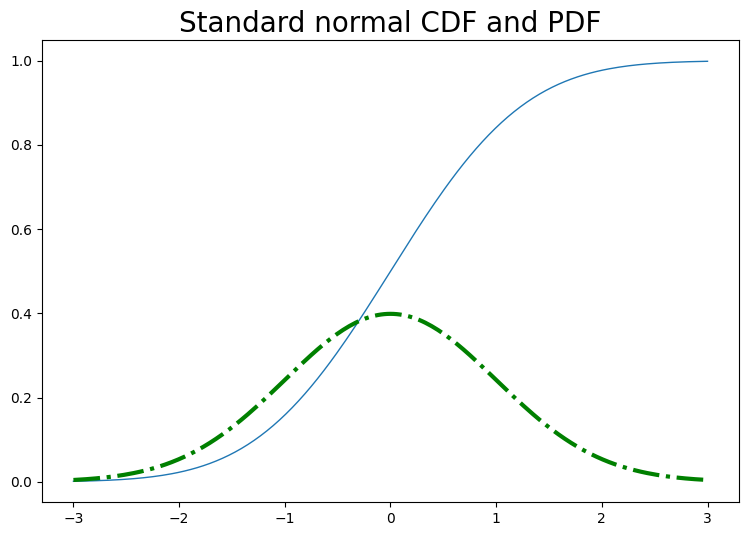

# Black-Scholes formulas
# call
# t is tau in the formula above
def bs_call(s, K, sigma, t, r=0, d=0):
    d1 = (log(s/K) + (r - d)*t)/(sigma*sqrt(t)) + sigma*sqrt(t)/2
    d2 = d1 - sigma*sqrt(t)
    
    c = s*exp(-d*t)*norm.cdf(d1) - K*exp(-r*t)*norm.cdf(d2)
    delta = exp(-d*t)*norm.cdf(d1)
    gamma = exp(-d*t)*norm.pdf(d1)/s/sigma/sqrt(t)
    
    return {'c': c, 'delta': delta, 'gamma': gamma}

#put
def bs_put(s, K, sigma, t, r=0, d=0):
    d1 = (log(s/K) + (r - d)*t)/(sigma*sqrt(t)) + sigma*sqrt(t)/2
    d2 = d1 - sigma*sqrt(t)
    
    p = K*exp(-r*t)*norm.cdf(-d2) - s*exp(-d*t)*norm.cdf(-d1)
    delta = -exp(-d*t)*norm.cdf(-d1)
    gamma = exp(-d*t)*norm.pdf(d1)/s/sigma/sqrt(t)
    
    return {'p': p, 'delta': delta, 'gamma': gamma}

print(bs_call(K=100, s=100, sigma=0.3, t=1))
print(bs_call(K=100, s=102, sigma=0.3, t=1))
print(bs_call(K=100, s=100, t=1, sigma=.3, r=0.05))
print(bs_call(s=100, K=90, t=1, sigma=.3))

{'c': 11.923538474048499, 'delta': 0.5596176923702425, 'gamma': 0.013149311030262966}
{'c': 13.068803286156744, 'delta': 0.5855095394527341, 'gamma': 0.012736690514019119}
{'c': 14.231254785985826, 'delta': 0.6242517279060125, 'gamma': 0.012647764437231514}
{'c': 17.0128799018497, 'delta': 0.6918854176337346, 'gamma': 0.011728453149086748}

# option price as a function of the underlying
K, sig, T, r = 100, 0.3, 1, 0.05 #0.02

# payoffs of call and put
payoff_c = lambda s, k: (s - k)*(s > k)
payoff_p = lambda s, k: (k - s)*(k > s)

# some temp functions
tmpc = lambda x: bs_call(x, K, sig, T, r)['c']
tmpp = lambda x: bs_put(x, K, sig, T, r)['p']
tmp_payoff_c = lambda x: payoff_c(x, K)
tmp_payoff_p = lambda x: payoff_p(x, K)

# plot
x = np.linspace(50, 150, 201)
plt.figure(figsize=(15, 6))
plt.subplot(1, 2, 1)
y = tmpc(x)
plt.plot(x, y, label='Black-Scholes')
y = tmp_payoff_c(x)
plt.plot(x, y, color='red', ls='dashed', label='payoff')
plt.xlabel(r'$S$', fontsize=15)
plt.ylabel('call price', fontsize=15)
plt.legend()
plt.subplot(1, 2, 2)
y = tmpp(x)
plt.plot(x, y, label='Black-Scholes')
y = tmp_payoff_p(x)
plt.plot(x, y, color='red', ls='dashed', label='payoff')
plt.xlabel(r'$S$', fontsize=15)
plt.ylabel('put price', fontsize=15)
plt.legend();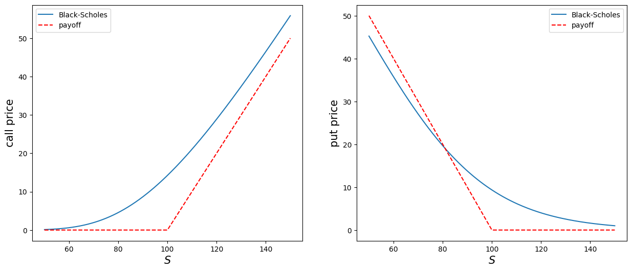

# option price as a function of strike
s, sig, T = 100, 0.3, 1

tmpc = lambda x: bs_call(s, x, sig, T)['c']
tmpp = lambda x: bs_put(s, x, sig, T)['p']

# plot
x = np.linspace(50, 150, 201)
plt.figure(figsize=(15, 6))
plt.subplot(1, 2, 1)
y = tmpc(x)
plt.plot(x, y, label='Black-Scholes')
plt.xlabel(r'$K$', fontsize=15)
plt.ylabel('call price', fontsize=15)
plt.subplot(1, 2, 2)
y = tmpp(x)
plt.plot(x, y, label='Black-Scholes')
plt.xlabel(r'$K$', fontsize=15)
plt.ylabel('put price', fontsize=15);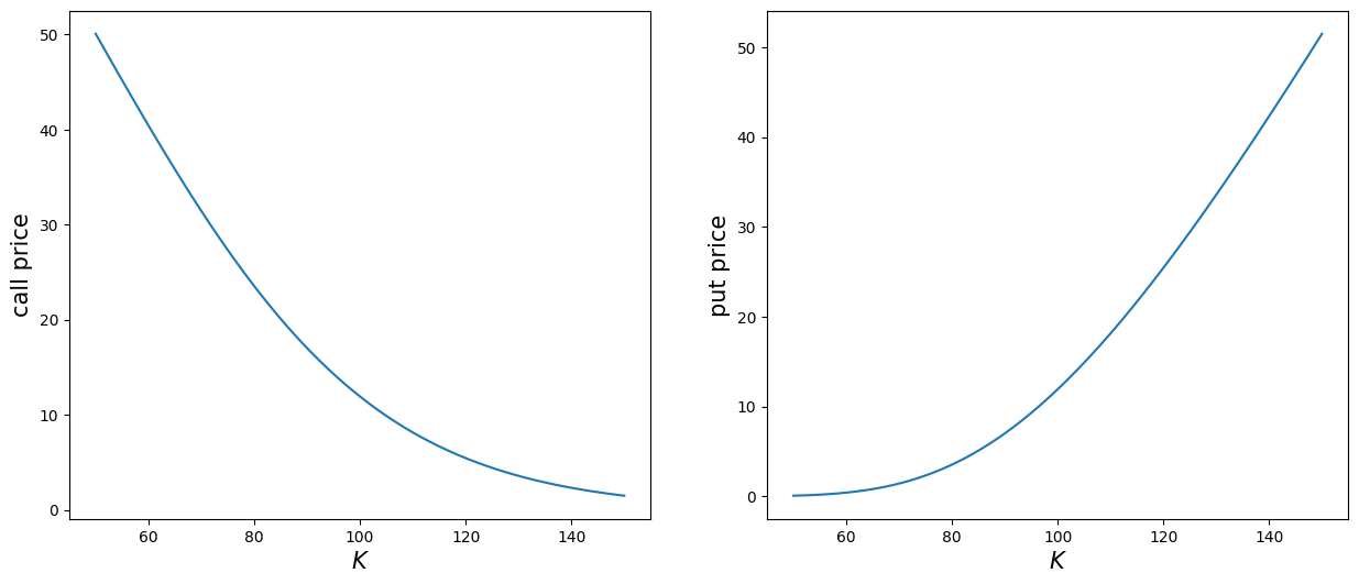

# option price as a function of volatility
s, K, T = 100, 95, 1

tmpc = lambda x: bs_call(s, K, x, T)['c']
tmpp = lambda x: bs_put(s, K, x, T)['p']

# plot
x = np.linspace(0.05, 1.5, 201)
plt.figure(figsize=(15, 6))
plt.subplot(1, 2, 1)
y = tmpc(x)
plt.plot(x, y, label='Black-Scholes')
plt.xlabel(r'$\sigma$', fontsize=15)
plt.ylabel('call price', fontsize=15)
plt.subplot(1, 2, 2)
y = tmpp(x)
plt.plot(x, y, label='Black-Scholes')
plt.xlabel(r'$\sigma$', fontsize=15)
plt.ylabel('put price', fontsize=15);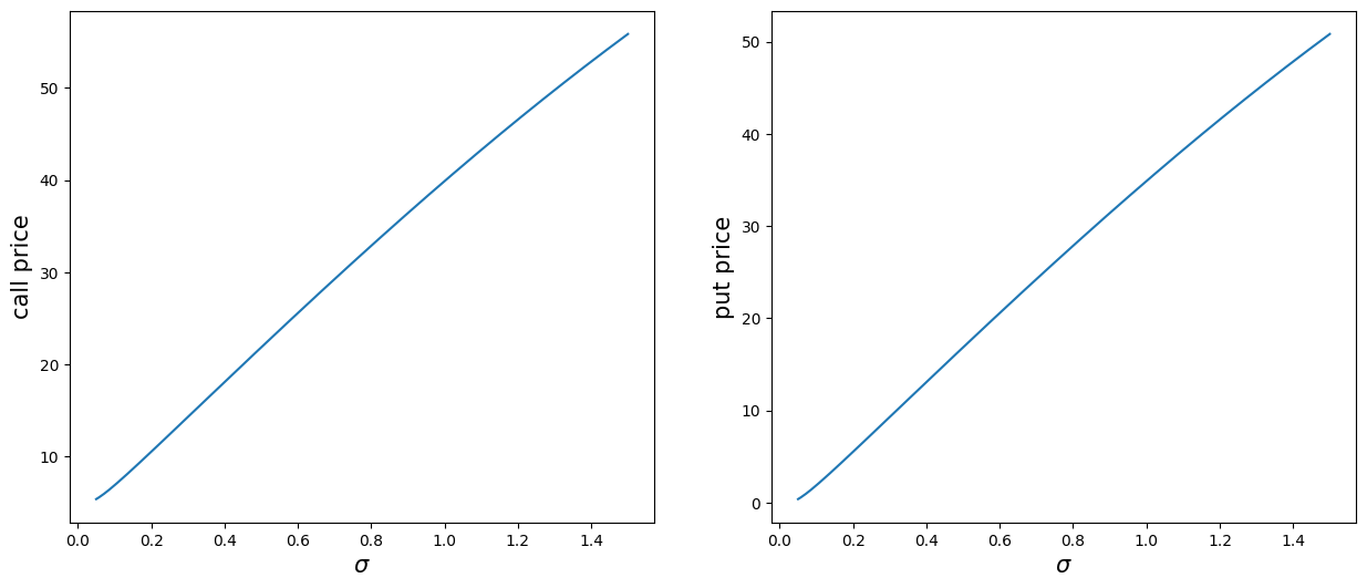

# option price as a function of time to expiry
s, K, sigma = 100, 102, 0.3

tmpc = lambda x: bs_call(s, K, sigma, x)['c']
tmpp = lambda x: bs_put(s, K, sigma, x)['p']

# plot
x = np.linspace(0.01, 2, 201)
plt.figure(figsize=(15, 6))
plt.subplot(1, 2, 1)
y = tmpc(x)
plt.plot(x, y, label='Black-Scholes')
plt.xlabel('Time to expiry', fontsize=15)
plt.ylabel('call price', fontsize=15)
plt.subplot(1, 2, 2)
y = tmpp(x)
plt.plot(x, y, label='Black-Scholes')
plt.xlabel('Time to expiry', fontsize=15)
plt.ylabel('put price', fontsize=15);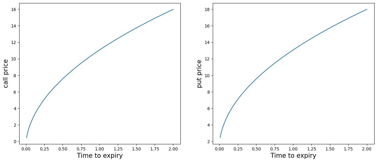

The Greeks

Sensitivities of option prices in Black-Scholes model - the Greeks.

Assume the dividend rate $d = 0$.

注: 股利率(dividend rate) 是指公司向股东支付的利润分配率, 在 Black-Scholes 模型中通常假设为 $0$.

For call:
- $\displaystyle \Delta_C = \frac{\p C}{\p S} = N(d_1)$
- Dual $\displaystyle \Delta_C^K = \frac{\p C}{\p K} = -e^{-rT} N(d_2)$
- $\displaystyle \Gamma = \frac{\p^2 C}{\p S^2} = \frac{n(d_1)}{S\sigma\sqrt T}$
- $\displaystyle \Theta_C = \frac{\p C}{\p T} = \frac{S \sigma}{2\sqrt T} n(d_1) + r K e^{-rT} N(d_2)$
- $\displaystyle \nu \, (\text{vega}) = \frac{\p C}{\p \sigma} = S \sqrt T \, n(d_1)$
- $\displaystyle \rho_C = \frac{\p C}{\p r} = K T e^{-rT} N(d_2)$
For put:
- $\displaystyle \Delta_P = \frac{\p P}{\p S} = \Delta_C - 1 = -N(-d_1)$
- Dual $\displaystyle \Delta_P^K = \frac{\p P}{\p K} = \Delta_C^K + e^{-r T} = e^{-rT} N(-d_2)$
- $\displaystyle \Gamma = \frac{\p^2 P}{\p S^2} = \frac{\p^2 C}{\p S^2}$
- $\displaystyle \Theta_P = \frac{\p P}{\p T} = \Theta_C - r e^{-rT} K = \frac{S \sigma}{2\sqrt T} n(d_1) - r K e^{-rT} N(-d_2)$
- $\displaystyle \nu \, (\text{vega}) = \frac{\p P}{\p \sigma} = \frac{\p C}{\p \sigma} = S \sqrt T n(d_1)$
- $\displaystyle \rho_P = \frac{\p P}{\p r} = \rho_C - T e^{-rT} K = -K T e^{-rT} N(-d_2)$

Note

$n(x) = N'(x)$ is the pdf for standard normal.
$\Theta_C > 0$, whereas $\Theta_P$ may be negative if $r > 0$.

Subtlety in self-financing

注: Subtlety = 区别. 此处探讨两种情况之细微区别:

投资者在每个时间步先调整投资组合
投资者先观察市场价格变化后再调整

Assume that all the tradings are done at the mid price $S_t$, i.e., no bid-ask spread and transaction cost.

注: mid price = 中间价, 即买入价和卖出价的平均值. 在实际交易中, 由于存在买卖差价(bid-ask spread)和交易成本, mid price 是一个理想化的假设.

In a discrete time setting, consider a portfolio consisting of holding $H_t$ shares of the underlying and $K_t$ dollars in the money/cash account at time $t$, interest and dividend are assumed zero for simplicity.

The monetary value $V_t$ of the portfolio, marked to market value at the mid price, is thus given by $V_t = H_tS_t + K_t$ (before the price of the underlying changes from $S_t$ to $S_{t+1}$). At this point, the investor may decide to change his portfolio before he observes the price change of the underlying from $S_t$ to $S_{t+1}$ or after the price change.

Before price change. In this case, the self-financing condition reads \[ V_t = H_t S_t + K_t = H_{t+1} S_t + K_{t+1}, \] where apparently $K_{t+1} = K_t + (H_t - H_{t+1}) S_t$. In other words, the investor simply moves his money from stock to money account (or the other way around) without pouring/withdrawing extra money/shares into/out of the portfolio. The value of the portfolio (after price change) at time $t+1$ is given by $V_{t+1} = H_{t+1}S_{t+1} + K_{t+1}$. Hence,

\[ \begin{aligned} \Delta V_{t+1} &= V_{t+1} - V_t \\ &= H_{t+1} S_{t+1} + K_{t+1} - (H_t S_t + K_t) \\ &= H_{t+1} S_{t+1} + K_{t+1} - (H_{t+1} S_t + K_{t+1}) \\ &= H_{t+1} \Delta S_{t+1}. \end{aligned} \]

If we write $H_{t+1} = H_t + \Delta H_{t+1}$, then

\[ \Delta V_{t+1} = H_t \Delta S_{t+1} + \Delta H_{t+1} \Delta S_{t+1} \]

After price change. In this case, the self-financing condition becomes \[ V_{t+1} = H_t S_{t+1} + K_t = H_{t+1} S_{t+1} + K_{t+1}, \] where $K_{t+1} = K_t + (H_t - H_{t+1}) S_{t+1}$. Hence, \[ \begin{aligned} \Delta V_{t+1} &= V_{t+1} - V_t \\ &= H_{t+1} S_{t+1} + K_{t+1} - (H_t S_t + K_t) \\ &= H_{t+1} S_{t+1} + K_t + (H_t - H_{t+1}) S_{t+1} - (H_t S_t + K_t) \\ &= H_t \Delta S_{t+1}. \end{aligned} \]

The subtlety results from the investor’s decision to rebalance his position before or after he observes the price change. Moreover, the discrepancy between the two increments of portfolio values is exactly the covariation between the holdings $H_t$ and the price $S_t$ of the underlying. In the continuous time limit, the discrepancy becomes insignificant should the covariation vanishes in the continuous time limit. In a recent paper by Carmona and Webster, the authors argued that, in the high frequency trading regime, empirically this covariation is statistically significant. As a result, the process of holdings $H_t$ cannot be of finite variation, counterintuitive to common knowledge.

即使在“无交易成本”的理想模型中, 投资者调仓的时机选择会对组合价值变化产生不同影响, 这种细微差异在连续时间极限中通常被忽略, 但在高频市场中却非常重要, 因为实际持仓路径和价格变动之间的协变并不为零.

Self-financing with traded price

In reality, trading incurs transaction cost which consist of bid-ask spread, fees, and taxes. The self-financing conditions with transaction cost becomes

Before price change. \[ V_t = H_t S_t + K_t = H_{t+1} S_t + K_{t+1} , \] where $K_{t+1} = K_t + (H_t - H_{t+1})S_t - c_t$ and $c_t > 0$ denotes the transaction cost at time $t$. Hence, the increment of $V$ at time $t+1$ \[ \begin{aligned} \Delta V_{t+1} &= V_{t+1} - V_t \\ &= H_{t+1} S_{t+1} + K_t + (H_t - H_{t+1}) S_t - c_t - (H_t S_t + K_t) \\ &= H_{t+1} \Delta S_{t+1} - c_t \\ &= H_t \Delta S_{t+1} + \Delta H_{t+1} \Delta S_{t+1} - c_t. \end{aligned} \]
After price change. By the same token, in this case one can show that \[ \Delta V_{t+1} = H_t \Delta S_{t+1} - c_{t+1} \]

where the transaction cost $c_{t+1}$ is incurred at time $t+1$.

Delta hedging

The portfolio used in deriving the Black-Scholes PDE is called delta-hedging.

利用 The Greeks 定义的 $\Delta$, Delta Hedging 就是构建一个投资组合, 使得这个组合整体的 $\Delta = 0$, 从而不受标的资产价格小幅变化影响.

Example: 假设你卖出了一个欧式看涨期权, 其 $\Delta = 0.6$; 那么你要买入 0.6 股标的资产来进行对冲.

Note

Rebalancing of hedging portfolio is done after the price change.

我们设 portfolio 为 $\pi = (s,c,o)$, 也就是 stock, cash, option.

\[ \pi^{\text{naked}} = (0,0,-1). \]

那么这个 naked portfolio 的价值为 $V(\pi^{\text{naked}})=-C$.

所以:

\[ \text{PNL}_{\text{naked}} = V(\pi^{\text{naked}}_{\text{tomorrow}}) - V(\pi^{\text{naked}}_{\text{today}}) = -C_{\text{tomorrow}} + C_{\text{today}}. \]

至于 delta hedging portfolio, 我们设 $\pi^{\text{delta}} = (x,0,-1)$.

那么:

\[ \Delta_{\pi^{\text{delta}}} = x - 0 - \Delta_C = x - N(d_1). \]

由于 $\Delta_{\pi^{\text{delta}}} = 0$, 所以 $x = N(d_1)$.

\[\begin{align*} V(\pi^{\text{delta}}_{\text{today}}) &= N(d_1) S_{\text{today}} - C_{\text{today}} \\ V(\pi^{\text{delta}}_{\text{tomorrow}}) &= N(d_1) S_{\text{tomorrow}} - C_{\text{tomorrow}} \\ \text{PNL}_{\text{delta}} &= V(\pi^{\text{delta}}_{\text{tomorrow}}) - V(\pi^{\text{delta}}_{\text{today}}) \\ \end{align*}\]

一个数值例子: 设 $\pi = (250, 10000, -200)$.

\[ V_{\pi} = 250 S + 10000 - 200 C = 250 \times 10 + 10000 - 200 \times 0.25 = 12450. \]

\[ \Delta_{\pi} = 250 + 0 - 200 \times 29\% = 192. \]

这就意味着你需要卖出 192 的股票.

An example on delta hedge

r, sigma = 0, 0.3 
s0, K = 10, 11
dt = 1/252 # one day 
t = 1/4 # a quarter of year, 3 month

# unpack a dict by using the .values method for dict object
c, delta, _ = bs_call(s0, K, sigma, t, r).values()
print(f'call price = {c}, delta = {delta}') 
bs_call(s0, K, sigma, t, r)

call price = 0.25002448066930727, delta = 0.28760290709660397

{'c': 0.25002448066930727,
 'delta': 0.28760290709660397,
 'gamma': 0.2273127644037836}

print(bs_call(s0, K, sigma, t, r))
print(bs_call(s0, K, sigma, t, r).values())

{'c': 0.25002448066930727, 'delta': 0.28760290709660397, 'gamma': 0.2273127644037836}
dict_values([0.25002448066930727, 0.28760290709660397, 0.2273127644037836])

# a range of underlying prices one day later
s = s0 + np.linspace(-1, 1, 21)
print(s)

bs_call(s, K, sigma, t-dt, r)['c']
delta*s0 - c

[ 9.   9.1  9.2  9.3  9.4  9.5  9.6  9.7  9.8  9.9 10.  10.1 10.2 10.3
 10.4 10.5 10.6 10.7 10.8 10.9 11. ]

2.6260045902967324

pnl_naked = c - bs_call(s, K, sigma, t-dt, r)['c']
pnl_delta = delta*s - bs_call(s, K, sigma, t-dt, r)['c'] - (delta*s0 - c)
pd.DataFrame({'naked': pnl_naked, 'delta_hedged': pnl_delta})

	naked	delta_hedged
0	0.189399	-0.098204
1	0.178589	-0.080254
2	0.166344	-0.063738
3	0.152554	-0.048768
4	0.137110	-0.035452
5	0.119905	-0.023896
6	0.100837	-0.014204
7	0.079807	-0.006474
8	0.056725	-0.000796
9	0.031504	0.002744
10	0.004069	0.004069
11	-0.025650	0.003111
12	-0.057711	-0.000190
13	-0.092164	-0.005883
14	-0.129050	-0.014009
15	-0.168397	-0.024596
16	-0.210225	-0.037664
17	-0.254544	-0.053222
18	-0.301352	-0.071269
19	-0.350638	-0.091795
20	-0.402383	-0.114780

# plot
plt.figure(figsize=(9, 6))
plt.plot(s, pnl_naked, 'o-', label='Naked call')
plt.plot(s, pnl_delta, 'o-.', color='orange', label='Delta hedged')
plt.hlines(y=0, xmin=min(s), xmax=max(s), ls='dashed')
plt.grid(color='grey', ls='dotted')
plt.ylabel('P&L', fontsize=15)
plt.xlabel(r'$s$', fontsize=15)
plt.legend();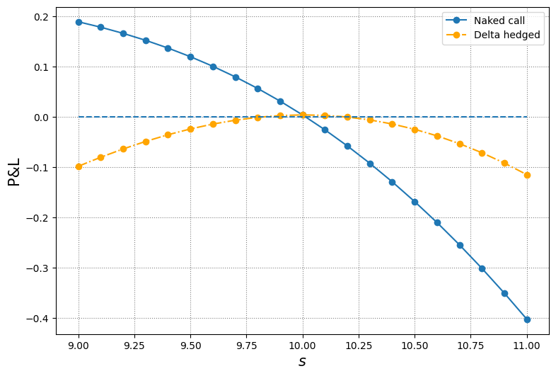

# zoom into the interval [9.5, 10.5]
plt.figure(figsize=(9, 6))
plt.plot(s, pnl_naked, 'o-', label='Naked call')
plt.plot(s, pnl_delta, 'o-.', color='orange', label='Delta hedged')
plt.hlines(y=0, xmin=min(s), xmax=max(s), ls='dashed')
plt.grid(color='grey', ls='dotted')
plt.ylabel('P&L', fontsize=15)
plt.xlabel(r'$s$', fontsize=15)
plt.xlim(9.5, 10.5)
plt.legend();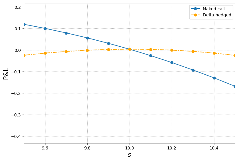

An example on delta-gamma hedge

Delta-gamma neutral: $\displaystyle \Delta = \frac{\partial C}{\partial S} = 0, \Gamma = \frac{\partial^2 C}{\partial S^2} = 0$.

\[ \Gamma_{\pi^{\text{naked}}} = -\frac{\partial^2 C}{\partial S^2} = -\Gamma_{\text{call}}. \]

为了保证 $\Gamma = 0$, 我们必须引入另一个用来对冲的 option.

\[ \pi = (\overset{\text{stock}}{x}, \overset{\text{cash}}{y}, \overset{\text{option}}{z}, \overset{\text{hedging option}}{w}). \]

\[\begin{align*} 0 = \Delta_{\pi} &= x + 0 + z \Delta_{\text{call}} + w \Delta_{\text{hedge}} \\ 0 = \Gamma_{\pi} &= 0 + 0 + z \Gamma_{\text{call}} + w \Gamma_{\text{hedge}}. \end{align*}\]

所以, 我们就有: $\displaystyle w = - \frac{\Gamma_{\text{call}}}{\Gamma_{\text{hedge}}}z$.

Note

The gammas of the underlying and forward are zero. To construct a delta-gamma hedge portfolio we need to add into the portfolio an instrument that has nonzero gamma, say, call or put options.

Delta-Gamma Hedging 是构造一个组合, 使得它对标的资产价格的一阶和二阶变化都不敏感.

现在假设有 $-1$ 单位的 $C$ (卖出 $C$), $x$ 单位的 $C_1$ (对冲工具), $y$ 单位的标的资产 (这里就是 stock).

$\displaystyle -\Gamma_C + x \Gamma_{C_1} = 0 \Longrightarrow x = \frac{\Gamma_C}{\Gamma_{C_1}}$
$\displaystyle C + x C_1 + y S$
$\displaystyle -\Delta_C + x \Delta_{C_1} + y = 0 \Longrightarrow y = \Delta_C - x \Delta_{C_1}$

r, sigma, K, s0 = 0, 0.3, 11, 10
dt, t = 1/252, 1/4

# target call
c, delta, gamma = bs_call(s0, K, sigma, t, r).values()

# call for hedging
K_hg = 14
c_hg, delta_hg, gamma_hg = bs_call(s0, K_hg, sigma, t, r).values()

# 1 day later
s = s0 + np.linspace(-1, 1, 21)
cs = bs_call(s, K, sigma, t-dt, r)['c']
pnl_naked = c - cs
pnl_delta = delta*s - cs - (delta*s0 - c)
delta_dg = delta - gamma/gamma_hg*delta_hg
gamma_dg = gamma/gamma_hg
pnl_dg = delta_dg*s + gamma_dg*bs_call(s, K_hg, sigma, t-dt, r)['c'] - cs - (delta_dg*s0 + gamma_dg*c_hg  - c)

# pandas.DataFrame for presentation
df = pd.DataFrame(np.array([pnl_naked, pnl_delta, pnl_dg]).transpose())
df.columns = ['naked', 'delta hedged', 'delta-gamma hedged']
df

	naked	delta hedged	delta-gamma hedged
0	0.189399	-0.098204	-0.025266
1	0.178589	-0.080254	-0.018913
2	0.166344	-0.063738	-0.013499
3	0.152554	-0.048768	-0.009028
4	0.137110	-0.035452	-0.005487
5	0.119905	-0.023896	-0.002840
6	0.100837	-0.014204	-0.001027
7	0.079807	-0.006474	0.000038
8	0.056725	-0.000796	0.000471
9	0.031504	0.002744	0.000423
10	0.004069	0.004069	0.000075
11	-0.025650	0.003111	-0.000354
12	-0.057711	-0.000190	-0.000607
13	-0.092164	-0.005883	-0.000389
14	-0.129050	-0.014009	0.000633
15	-0.168397	-0.024596	0.002832
16	-0.210225	-0.037664	0.006620
17	-0.254544	-0.053222	0.012447
18	-0.301352	-0.071269	0.020799
19	-0.350638	-0.091795	0.032197
20	-0.402383	-0.114780	0.047194

# plot
plt.figure(figsize=(9, 6))
plt.plot(s, pnl_naked, 'o-', label='Naked call')
plt.plot(s, pnl_delta, 'o-.', color='orange', label='Delta hedged')
plt.plot(s, pnl_dg, 'o-.', color='red', label='Delta Gamma hedged')
plt.hlines(y=0, xmin=min(s), xmax=max(s), ls='dashed')
plt.grid(color='grey', ls='dotted')
plt.ylabel('P&L', fontsize=15)
plt.xlabel(r'$s$', fontsize=15)
plt.legend();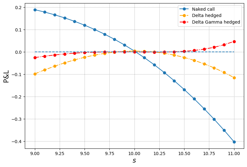

# zoom into the interval [9.5, 10.5]
plt.figure(figsize=(9, 6))
plt.plot(s, pnl_naked, 'o-', label='Naked call')
plt.plot(s, pnl_delta, 'o-.', color='orange', label='Delta hedged')
plt.plot(s, pnl_dg, 'o-.', color='red', label='Delta Gamma hedged')
plt.hlines(y=0, xmin=min(s), xmax=max(s), ls='dashed')
plt.grid(color='grey', ls='dotted')
plt.ylabel('P&L', fontsize=15)
plt.xlabel(r'$s$', fontsize=15)
plt.xlim(9.5, 10.5)
plt.legend();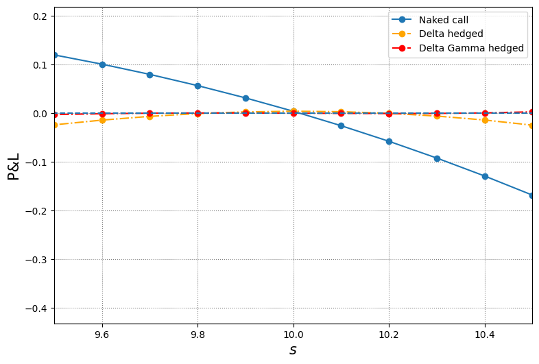

Dynamical hedging

As market conditions evolve, to maintain the delta neutrality of the portfolio, ideally we should dynamically change the holdings in the portfolio.

Only delta neutrality, not delta-gamma neutrality.

Note

Rebalancing of hedging portfolio is done after observing the price change.

An example on dynamical hedging

# parameters
r, sigma = 0, 0.3
s0, K = 10, 11
dt, t, days_forward = 1/252, 1/4, 30

# portfolio positions in cash, options, underlying
# x : number of shares in underlying
# y : dollars in cash
# z : number of options

# short 1000 calls
z = -1000

# current price and delta of call
c, delta, _ = bs_call(s0, K, sigma, t, r).values()

# construct a zero value and delta neutral portfolio
x = delta*(-z)
y = -(x*s0 + z*c)
port_value, port_delta = x*s0 + y + z*c, x + z*delta
s, pnl_cum = s0, 0

# pandas.DataFrame for presentation
pd.DataFrame(np.array([port_value, port_delta, pnl_cum, s, c, x, y, z*delta]).reshape(1, 8))

	0	1	2	3	4	5	6	7
0	-8.526513e-14	0.0	0.0	10.0	0.250024	287.602907	-2626.00459	-287.602907

# 1 day later
i = 1
s_new = s0*exp((r - sigma**2/2)*dt + sigma*sqrt(dt)*norm.rvs()) # sample a new stock price
c_new, delta_new, _ = bs_call(s_new, K, sigma, t-i*dt, r).values()

# portfolio value before rebalance 
port_value_new = x*s_new + y*exp(r*i*dt) + z*c_new
pnl_cum = pnl_cum + port_value_new - port_value

# rebalance to delta neutral
x_new = delta_new*(-z)
y_new = y*exp(r*i*dt) + (x - x_new)*s_new
port_value = x_new*s_new + y_new + z*c_new
port_delta = x_new + z*delta_new
s, c, x, delta, y = s_new, c_new, x_new, delta_new, y_new


# display the result
pd.DataFrame(np.array([port_value, s, c, y, x]).reshape(1, 5),
            columns=['portfolio value', 'stock price', 'call price', 'shares', 'cash'])

	portfolio value	stock price	call price	shares	cash
0	2.546886	9.892218	0.216479	-2367.146177	261.435023

# Let's see how it works for 30 days forward
# initialize data
port_value = np.zeros(days_forward+1)
s = s0 + np.zeros(days_forward+1)
calls = c + np.zeros(days_forward+1)
deltas = delta + np.zeros(days_forward+1)
shares = x + np.zeros(days_forward+1)
cash = y + np.zeros(days_forward+1)

for i in range(days_forward):    
    # sample a stock price
    s[i+1] = s[i]*exp((r - sigma**2/2)*dt + sigma*sqrt(dt)*norm.rvs()) 
    
    # calculate new call price and delta
    calls[i+1], deltas[i+1], _ = bs_call(s[i+1], K, sigma, t-i*dt, r).values()
    
    # portfolio value before rebalance 
    port_value[i+1] = shares[i]*s[i+1] + cash[i]*exp(r*dt) + z*calls[i+1]
    
    # rebalance (self-financing) to delta neutral
    shares[i+1] = deltas[i+1]*(-z)
    cash[i+1] = cash[i]*exp(r*dt) + (shares[i] - shares[i+1])*s[i+1]
    
# display the result
df = pd.DataFrame(np.array([port_value, s, calls, shares, cash]).T)
df.columns = ['portfolio value', 'stock price', 'call price', 'shares', 'cash']
df

	portfolio value	stock price	call price	shares	cash
0	0.000000	10.000000	0.216479	261.435023	-2367.146177
1	-1.685025	9.942157	0.233767	274.561382	-2497.650498
2	2.268928	9.941718	0.229692	272.461998	-2476.779020
3	6.211547	9.932415	0.223215	268.327792	-2435.716366
4	7.977730	9.800739	0.186117	237.182288	-2130.467417
5	11.198113	9.743563	0.169335	222.740773	-1989.755598
6	11.639786	9.924673	0.209234	260.177939	-2361.307222
7	8.445821	9.679310	0.148590	204.653243	-1823.866480
8	4.882468	9.424510	0.100008	153.308707	-1339.969360
9	5.726561	9.286795	0.078051	127.580670	-1101.038366
10	7.598509	9.388071	0.089100	141.955984	-1235.994839
11	10.324611	9.406149	0.088940	142.546174	-1241.546252
12	10.635569	9.585027	0.114127	173.031658	-1533.750432
13	10.375330	9.783245	0.148685	211.536361	-1910.451358
14	9.859347	9.595023	0.109386	169.590464	-1507.979495
15	12.248389	9.514560	0.093351	151.388201	-1334.792971
16	7.022855	9.221413	0.054197	99.998587	-860.908107
17	9.182860	9.267979	0.056694	104.264357	-900.443174
18	11.500153	9.296259	0.057325	105.861646	-915.291984
19	-2.567556	9.746510	0.119057	186.474293	-1700.983964
20	1.108896	9.776974	0.121061	190.090952	-1736.343949
21	3.292136	9.669038	0.098361	163.857148	-1482.688290
22	-1.645460	9.389589	0.057509	109.119273	-968.722121
23	0.884305	9.384055	0.054375	105.194186	-931.888885
24	3.350541	9.372953	0.050741	100.368375	-886.656788
25	5.651420	9.440110	0.055180	108.085315	-959.505545
26	7.572448	9.363605	0.044990	92.697566	-815.420747
27	9.973373	9.384116	0.044491	92.648530	-814.960587
28	11.436208	9.290807	0.034383	75.986501	-660.156885
29	13.356387	9.365511	0.038139	83.349842	-729.118332
30	15.200208	9.307130	0.031429	71.947088	-622.991417

Dynamic hedge in practice

Continuous trading in practice is unrealistic.
The tradeoff between frequency of rebalancing and replication of derivative
Imperfect hedge, risk penalty
Transaction cost, market order or limit order, etc

注: Replication creates an asset or portfolio using a combination of another asset, portfolio, and/or derivative. The following combinations produce the equivalent single asset: Long asset + Short derivative = Long risk free asset.

Deep hedging

Research works on hedging problem that resort to reinforcement learning techniques include

Halperin, QLBS: Q-Learner in the Black-Scholes(-Merton) Worlds
Buehler, Gonon, Teichmann, and Wood, Deep hedging
Cao, Chen, Hull, and Poulos, Deep hedging of derivatives using reinforcement learning
Kolm and Ritter, Dynamic replication and hedging: a reinforcement learning approach

Deep hedging in a nutshell

The key idea behind deep hedging in the aforementioned works is to formulate the hedging problem as a stochastic control problem with certain objective functional, then solve the resulting control problem by the techniques introduced in reinforcement learning.

Let’s take the work by Cao, Chen, Hull, and Poulos as an example.

Notations

$i$: time, running from $0$ to $n$
$C_i$: value of the call/derivative at the beginning of the time $i$
$S_i$: price of the underlying at the beginning of the time $i$
$H_i$: holdings of the underlying between time $i$ and $i+1$.
$\kappa$: proportional transaction cost
$R_i$: running reward gained at time $i$

Settings in Cao-Chen-Hull-Poulos

Cao-Chen-Hull-Poulos formulate the hedging problem as follows.

a trader is hedging a short position in a call option
hedging portfolio consisting of shares in the underlying, no cash component?
the trader re-balances his position at time intervals of length $\Delta t$ and is subject to trading costs
The life of the option is $n$.
The cost of a trade in the underlying asset is proportional to the value of what is being bought or sold
The state at time $i$ is defined by three parameters:
1. The holding $H_{i-1}$ of the asset during the previous time period; i.e., from time $i-1$ to time $i$
2. The asset price $S_i$ at time $i$
3. The time to maturity $(n-i)$
The action/control $H_i$ at time $i$ is the amount of the asset to be held for the next period, i.e., from time $i$ to time $i+1$.
Rebalance is done after observing the price change.

Two alternative formulations

There are two alternative formulations for the hedging problem:
- the accounting P&L formulation
- the cash flow formulation.
For ease of exposition, no discounting is assumed in the control problem, i.e., $\gamma=1$

Accounting P&L formulation

For $1 \leq i \leq n$, define the running reward gained at time $i$ as

\[ \begin{aligned} R_i &= -C_i + C_{i-1} + H_{i-1} (S_i - S_{i-1}) - \kappa |S_i (H_i - H_{i-1})| \\ &= -\Delta C_i + \underbrace{H_{i-1} \Delta S_i}_{\text{marked to market}} - \underbrace{\kappa |S_i \Delta H_i|}_{\text{transaction cost}}. \end{aligned} \]

Note that this formulation is consistent with the self-financing condition with transaction cost that was discussed previously. To set up the hedging initially and liquidate the position at expiry of option, we add to the (undiscounted) cumulative rewards

initial reward: $-\kappa|S_0 H_0|$
terminal reward: $-\kappa|S_n H_n|$

Thus, the performance criterion $Y^A$ for a given hedging strategy $(H_0, \cdots, H_n)$ reads

\[ \begin{aligned} Y^A &= -\kappa |S_0 H_0| + \sum_{i=1}^n R_i - \kappa |S_n H_n| \\ &= -\kappa |S_0 H_0| + C_0 - C_n + \sum_{i=1}^n H_{i-1} \Delta S_i - \kappa \sum_{i=1}^n |S_i \Delta H_i| - \kappa |S_n H_n|. \end{aligned} \]

Cashflow formulation

In this formulation, for $1 \leq i \leq n$, the running reward gained at time $i$ is defined by

\[ R_i = S_i(H_{i-1} - H_i) - \kappa |S_i(H_i - H_{i-1})| = -S_i \Delta H_i - \kappa |S_i \Delta H_i| \]

with - initial cost for setting up a position: $-S_0H_0 - \kappa|S_0 H_0|$ - terminal cost for liquidate the position and payoff to call: $S_nH_n - \kappa|S_n H_n| - C_n$.

Thus, the performance criterion $Y^C$ for a given hedging strategy $(H_0, \cdots, H_n)$ reads

\[ \begin{aligned} Y^C &= -S_0 H_0 - \kappa |S_0 H_0| + \sum_{i=1}^n R_i + S_n H_n - \kappa |S_n H_n| - C_n \\ &= -S_0 H_0 - \kappa |S_0 H_0| - \sum_{i=1}^n S_i \Delta H_i - \kappa \sum_{i=1}^n |S_i \Delta H_i| + S_n H_n - \kappa |S_n H_n| - C_n. \end{aligned} \]

Accounting P&L vs cashflow

Recall that

\[ \begin{aligned} Y^A &= -\kappa |S_0 H_0| + C_0 - C_n + \sum_{i=1}^n H_{i-1} \Delta S_i - \kappa \sum_{i=1}^n |S_i \Delta H_i| - \kappa |S_n H_n| \\ &= -\kappa |S_0 H_0| + C_0 - C_n + H_n S_n - H_0 S_0 - \sum_{i=1}^n S_i \Delta H_i - \kappa \sum_{i=1}^n |S_i \Delta H_i| - \kappa |S_n H_n|. \end{aligned} \]

where in the last equality we applied the following summation by parts formula

\[ \sum_{i=1}^n H_{i-1} \Delta S_i = H_n S_n - H_0 S_0 - \sum_{i=1}^n S_i \Delta H_i. \]

It follows that

\[ Y^A - Y^C = C_0. \]

The two formulations are basically the same.

Objective functional and resulting control problem

Objective functional for the performance criterion $Y$ is given by its expectation penalized by a risk measure. Namely,

\[ \Eof{Y} - \lambda \rho(Y), \]

where $\rho$ is certain prespecified risk measure. Hence, the hedging problem can be recast as the following stochastic control problem

\[ \max_{(H_0, \cdots, H_n)} \Eof{Y} - \lambda \rho(Y). \]

From this point on, reinforcement learning techniques are then applied to solve the above control problem.

Note

In the original Cao-Chen-Hull-Poulos paper, the authors chose to penalize the expected reward by standard deviation. However, from control theory point of view, penalizing expected reward by variance/standard deviation will induce (unnecessary?) difficulty due to time inconsistency.
In the Buehler et al paper, the authors utilized the expected shortfall or conditional value-at-risk as the risk measure.

Implementation of Deep hedging in `Tensorflow`

Courtsey: Laura He and Tony Xie, Baruch MFE 2020

Deep-hedging implementation with DDPG Algorithm

Step 1 Initialize neural network of $Q_1(s,a|\theta^{Q_1}), Q_2(s,a|\theta^{Q_2})$ and policy function $\mu(s|\theta^\mu)$. Set target networks $Q_1' \leftarrow Q_1,Q_2' \leftarrow Q_2,\mu' \leftarrow \mu$. Create replay buffer $R$.

Step 2 Begin loop:

for episode $= 1$ to n_path:

Generate random process ${N_i}, i = 0, 1, ..., m$ for action exploration.
Get initial state: $s_0 = [S_0$(stock price), $V_0$(option price), $H_{-1} = 0$(holding), $\tau_0 = T = m\, \mathrm{d}t$(time to maturity)$]$.

for $i = 0$ to $m$ ($m$ time intervals):

Step 2.1 Calculate action: $a_i = (1-\epsilon_i)\mu(s_i|\theta^\mu) + \epsilon_i N_i,\,\, s_i = [S_i, V_i, H_{i-1}, \tau_i = (m-i)\mathrm{d}t]$
Step 2.2 Execute $a_i$. Get $r_i = -(V_{i+1} - V_i) + H_i(S_{i+1} - S_i) - \kappa |S_ia_i|,\,\, 0\leqslant i<m$
$\hspace{4.2 cm} r_m = - \kappa|S_mH_{m-1}|$
Step 2.3 Observe new state: $s_{i+1} = [S_{i+1}, V_{i+1}, H_i = H_{i-1}+a_i, \tau_{i+1} = (m-i-1)\mathrm{d}t]$
Step 2.4 Store $(s_i, a_i, r_i, s_{i+1})$ in the replay buffer $R$.
Step 2.5 Sample $J$ transitions from $R$, mark as $(s_j, a_j, r_j, s_{j+1}), \,\, j = 1 \sim N/ J?$
$\hspace{1.6 cm}y_j^{(1)} = r_j + \gamma Q_1'(s_{i+1}, \mu'(s_{i+1}|\theta^{\mu'})|\theta^{Q'})$

$y_j^{(2)} = r_j^2 + ^2 Q_2’(s_{i+1}, ‘(s_{i+1}|^{’})|{Q’}) + 2 r_j Q_1’(s_{i+1}, ‘(s_{i+1}|^{’})|{Q’}) $

$\hspace{1.4 cm}$ Update $Q_{1,2}$: $Q_{1,2} = \underset{Q_{1,2}}{\mathrm{argmin}}\left\{\frac{1}{J}\sum_j\left(y_j^{(1,2)} - Q_{1,2}(s_j,a_j|\theta^{Q_{1,2}})\right)^2\right\}$
$\hspace{1.4 cm}$ Update $\mu$ using gradient descent: $\nabla_{\theta^{\mu}}G = \frac{1}{J}\sum_j\nabla_aF(s_j, a_j|\theta^{Q_{1,2}})\nabla_{\theta^{\mu}}\mu(s_j|\theta^{\mu}),\,\, \theta^\mu = \theta^\mu - \nabla_{\theta^\mu}G \times \text{step}$

Step 2.6 Update the target networks: $\theta^{Q'_{1,2}} \leftarrow \tau\theta^{Q_{1,2}} + (1-\tau)\theta^{Q'_{1,2}}, \,\,\theta^{\mu'} \leftarrow \tau\theta^\mu + (1-\tau)\theta^{\mu'}$

pip show DDPG

Note: you may need to restart the kernel to use updated packages.

WARNING: Package(s) not found: DDPG

# import DDPG and other related packages

import numpy as np
from DDPG.world import World
import tensorflow as tf
from DDPG.blackscholesgenerator import GenerateBSPath, BSCall
import matplotlib.pyplot as plt
import pandas as pd
import seaborn as sns

Performance of deep hedging vs delta hedging

# python function to implement the trained model 
def DDPG(n_path=5000, m=4, T=1/12, r=0, q=0, sigma=0.2, S0=100, K=100, model_path=""):
    stock_price, call_price, call_delta = GenerateBSPath(n_path=n_path, \
                m=m, T=T, r=r, q=q, sigma=sigma, S0=S0, K=K)
        
    V0 = call_price[0,0]
    initial_state = np.array([S0, V0, 0, T])
    state_size, action_size = 4, 1

    world = World(state_size, action_size, initial_state, dt=T/m)
    # load-in saved (trained) model 
    # actor_model = tf.keras.models.load_model(f'{model_path}/Actor_Model', compile=False)
    actor_model = tf.keras.layers.TFSMLayer(
        f'{model_path}/Actor_Model', 
        call_endpoint='serving_default'
    )

    actions_model = np.zeros((n_path, m))
    rewards = np.zeros(n_path)

    for episode in range(n_path):

        if episode % 2000 == 0:
            print(episode)

        world.initialize()

        for i in range(m):
            state = world.get_state()
            output = actor_model(np.array([state])) # 假设 output 是字典
            first_value = next(iter(output.values())).numpy()[0, 0]  # 提取第一个值并转为标量
            actions_model[episode, i] = first_value
            # actor_model(np.array([state]))[0,0]
            next_state, reward, done = world.act(actions_model[episode, i], (stock_price[episode, i+1], call_price[episode, i+1]))
            rewards[episode] += reward 

        state = world.get_state()
        rewards[episode] += world.act(0, (0,0))[1]

#    print(actions_model)
    
    positions = call_delta[:,:m]
    actions = np.hstack((call_delta[:,0].reshape(n_path,1), np.diff(call_delta[:,:m], axis = 1)))
    payoff = positions*np.diff(stock_price, axis=1) - np.diff(call_price, axis=1) - np.abs(actions*stock_price[:,:m])*0.01 
    payoff = np.sum(payoff, axis=1)
    payoff -= np.abs(call_delta[:,m]*stock_price[:,m])*0.01
        
    payoff_zero = - np.diff(call_price, axis = 1) 
    payoff_zero = np.sum(payoff_zero, axis = 1)
    
    hedging_cost_mean = np.array([-rewards.mean(), -payoff.mean(), -payoff_zero.mean()])
    hedging_cost_std = np.array([rewards.std(), payoff.std(), payoff_zero.std()])
    obj_func = hedging_cost_mean + 1.5*hedging_cost_std
    
    method_name = ["DDPG", "Delta", "No Hedge"]
    hedging_cost_mean = np.array([-rewards.mean(), -payoff.mean(), -payoff_zero.mean()])
    hedging_cost_std = np.array([rewards.std(), payoff.std(), payoff_zero.std()])
    obj_func = hedging_cost_mean + 1.5*hedging_cost_std
    
    mean_in_price = 100 * hedging_cost_mean / V0
    std_in_price = 100 * hedging_cost_std / V0
    obj_func_in_price = mean_in_price + 1.5*std_in_price
    
    result = pd.DataFrame({'Name': method_name,
                           'Mean': hedging_cost_mean,
                           'STD': hedging_cost_std, 
                           'Obj Func': obj_func, #\
                           'Mean in Option Price(%)': mean_in_price, 
                           'STD in Option Price(%)': std_in_price, #\
                           'Obj Func in Option Price(%)': obj_func_in_price})
    
    print(f"----------- DDPG Result: {m} hedges in {int(T*12)} month. -----------")
        
    print(result)
    
    plt.figure(figsize=(8,6))
    sns.histplot(rewards, label='DDPG', kde=True, stat='density', element='step')
    sns.histplot(payoff, kde=True, label='Delta', stat='density', color='orange', element='step')
    plt.legend()
    plt.show()
    
    return actor_model

# function for plotting optimal policy 
from mpl_toolkits.mplot3d import Axes3D

def plotAction(curr_model):
    
    TT = np.arange(0, 1, 0.05)
    SS = np.arange(80, 120, 0.5)
    Y, X = np.meshgrid(TT, SS)
    Z_DDPG = np.zeros((SS.shape[0], TT.shape[0]))
    #Z_BS = np.zeros((SS.shape[0], TT.shape[0]))

    for i in range(SS.shape[0]):
        for j in range(TT.shape[0]):
            BS_model = BSCall(T=TT[j], sigma=sigma, S0=SS[i])
            output = curr_model(np.array([[SS[i],BS_model[0],0,TT[j]]]))
            Z_DDPG[i,j] = next(iter(output.values())).numpy()[0][0]
            #Z_BS[i,j] = BS_model[1]
        
    V0 = BSCall(T=T, sigma=sigma, S0=S0)[0]
    BS_action_pos = [next(iter(curr_model(np.array([[S0, V0, _pos, T]])).values())).numpy()[0][0] for _pos in np.arange(-1,1,0.05)]
    
    # %matplotlib notebook
    fig = plt.figure(figsize=(16,6))  
    ax3 = fig.add_subplot(1, 2, 1, projection='3d')
    ax3.plot_surface(X, Y, Z_DDPG)
    # ax3.plot_surface(X,Y,Z_BS)
    plt.title("Action vs. Stock price & Time to maturity")
    plt.xlabel("Stock price")
    plt.ylabel("Time to maturity")
    
    ax2 = fig.add_subplot(1, 2, 2)
    ax2.plot(np.arange(-1, 1, 0.05), BS_action_pos)
    plt.title("Action vs. Position")
    plt.xlabel("Position")
    plt.show();

One-month option, weekly hedging

%%time
# model paramters
r, q, sigma, S0, K = 0, 0, 0.2, 100, 100

# simulation parameters
# option expires in a month, hedging weekly
T, m, n_path = 1/12, 4, 5_000

model_path = "DDPG/trained_models/1m/weekly"

# set random seed for reproducing the result
np.random.seed(9999)

weekly = DDPG(n_path=n_path, m=m, T=T, r=r, q=q, sigma=sigma, S0=S0, K=K, model_path=model_path)

0
2000
4000
----------- DDPG Result: 4 hedges in 1 month. -----------
       Name      Mean       STD  Obj Func  Mean in Option Price(%)  \
0      DDPG  1.135191  2.199476  4.434405                49.292365   
1     Delta  1.543443  1.172043  3.301507                67.019524   
2  No Hedge  0.053613  3.528923  5.346998                 2.327991   

   STD in Option Price(%)  Obj Func in Option Price(%)  
0               95.505890                   192.551201  
1               50.892563                   143.358369  
2              153.233282                   232.177914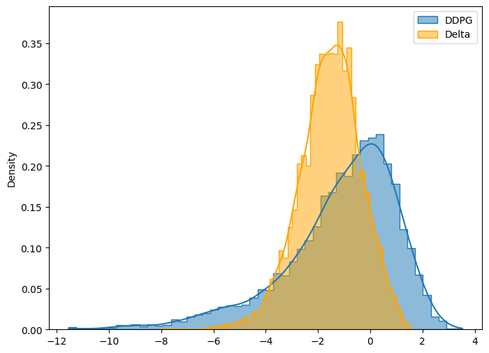

CPU times: total: 3.03 s
Wall time: 23.8 s

What does the optimal action look like?

plotAction(weekly)

One-month option, tridaily hedging

%%time
# one month option, tridaily hedging
T, m = 1/12, 10
model_path = "DDPG/trained_models/1m/3-day"
tridaily = DDPG(n_path=n_path, m=m, T=T, r=r, q=q, sigma=sigma, S0=S0, K=K, model_path=model_path)

0
2000
4000
----------- DDPG Result: 10 hedges in 1 month. -----------
       Name      Mean       STD  Obj Func  Mean in Option Price(%)  \
0      DDPG  1.798405  2.092016  4.936429                78.090545   
1     Delta  1.957786  0.940487  3.368517                85.011175   
2  No Hedge  0.017840  3.497339  5.263849                 0.774652   

   STD in Option Price(%)  Obj Func in Option Price(%)  
0               90.839724                   214.350131  
1               40.837944                   146.268091  
2              151.861840                   228.567411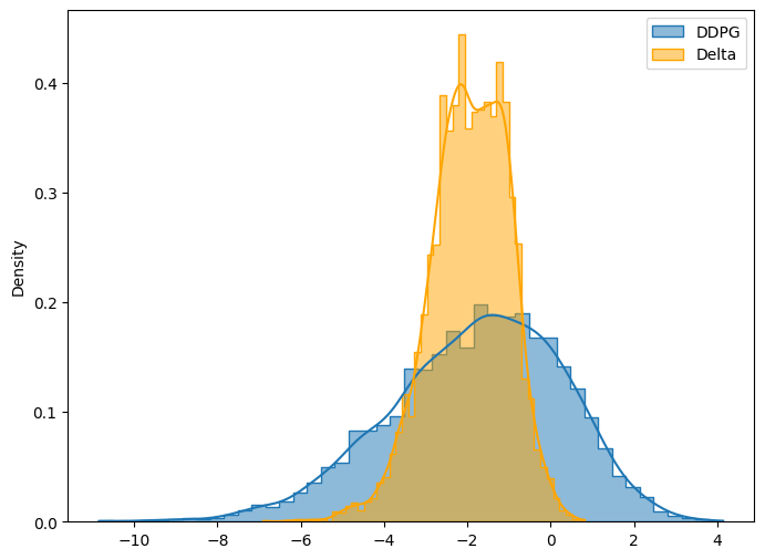

CPU times: total: 7.06 s
Wall time: 53.4 s

# plot tridaily action function 
plotAction(tridaily)

3-month option, weekly hedging

%%time
# 3 months option, weekly hedging
T, m = 3/12, 4
model_path = "DDPG/trained_models/3m/weekly"
weekly_3m = DDPG(n_path=n_path, m=m, T=T, r=r, q=q, sigma=sigma, S0=S0, K=K, model_path=model_path)

0
2000
4000
----------- DDPG Result: 4 hedges in 3 month. -----------
       Name      Mean       STD  Obj Func  Mean in Option Price(%)  \
0      DDPG  0.857973  3.904091  6.714109                21.515145   
1     Delta  1.474011  1.784586  4.150890                36.963365   
2  No Hedge -0.124989  6.013195  8.894803                -3.134323   

   STD in Option Price(%)  Obj Func in Option Price(%)  
0               97.901820                   168.367874  
1               44.751576                   104.090729  
2              150.791253                   223.052557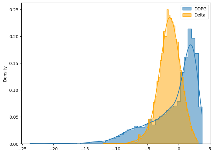

CPU times: total: 2.89 s
Wall time: 19.6 s

plotAction(weekly_3m)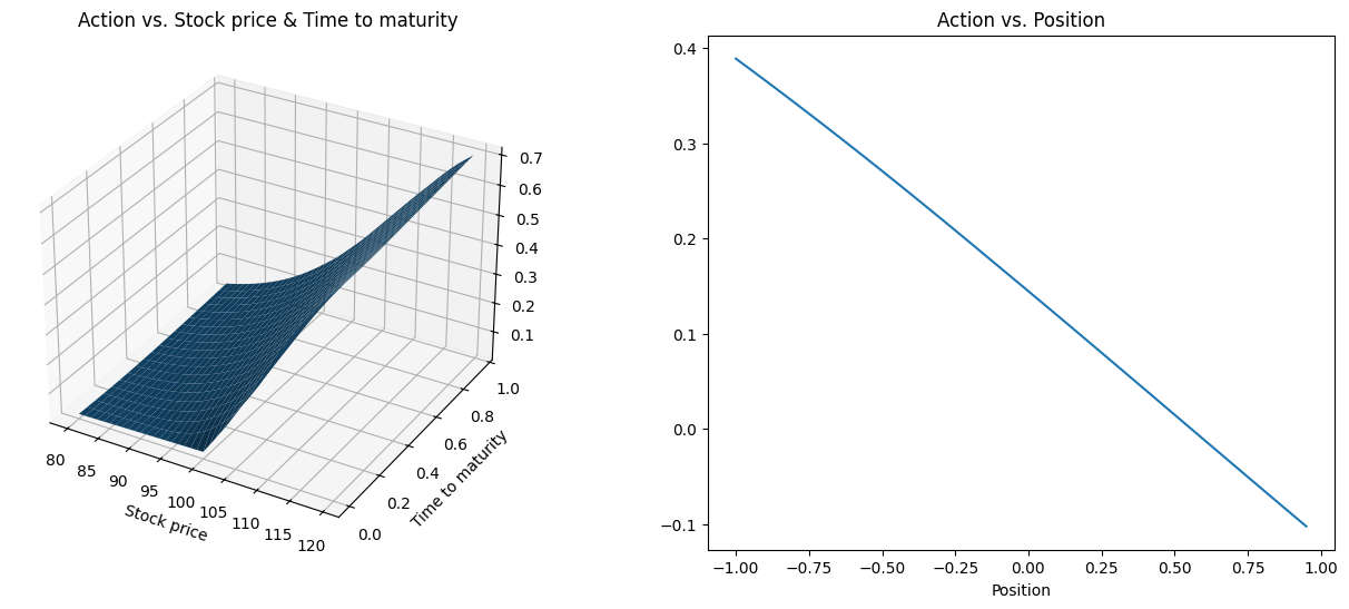

Concluding remarks on deep hedging

Hedging with DDPG Algorithm can reduce the average hedging cost, however, it increases the variance of cost for the Black-Scholes model and probably also for stochastic volatility models.
As is mentioned in the original paper, the impact of trading costs (or transaction cost) is to under-hedge relative to delta hedging in some situations and over-hedge in other situations. By hedging short European call option position, we observe under-hedge relative to delta hedging.
One may be able to reduce the variance of hedging cost in the DDPG Algorithm by adding more paths for training. In the code, we used 5000 training paths for each model while renewing the model after each episode. However, using too many paths in the training stage may result in overfitting.

Lecture Notes

Thanks to 段凤仪 (Duàn Fèng Yí) and 刘弘锌 (Liú Hóng Xīn) for their lecture notes.

Black-Scholes Model

Revolutionary Concept: The Black-Scholes model, developed 24 years ago, introduced groundbreaking ideas that transformed option pricing. It challenged traditional static hedging approaches with dynamic hedging, emphasizing continuous position adjustment.
New Ideas: Key concepts include delta hedging, where the number of shares held ($\Delta$) equals the partial derivative of the option price with respect to the stock price ($\displaystyle \frac{\partial C}{\partial S}$). This approach aims to make the portfolio risk-free.

模型假设:

Stock Price Movement: The model assumes that stock prices follow a geometric Brownian motion, where the return (change in price over price) follows a normal distribution. This assumption simplifies the pricing process.
Risk-Neutral Pricing: When pricing options, the model assumes a risk-neutral environment, where the expected return on the stock is equal to the risk-free interest rate. This assumption allows for consistent pricing across different market conditions.

Option Pricing with the Black-Scholes Model

Pricing Formula

Call Option Price: The formula for call option price is

\[ C = S e^{-D \tau} N(d_1) - K e^{-r \tau} N(d_2), \]

where $S$ is the stock price, $K$ is the strike price, $D$ is the dividend rate, $r$ is the risk-free interest rate, $\tau$ is the time to expiration, and $N(d_1)$ and $N(d_2)$ are the cumulative distribution functions of the standard normal distribution.

Put Option Price: The put option price formula is

\[ P = K e^{-r \tau} N(-d_2) - S e^{-D \tau} N(-d_1). \]

Parameter Estimation

Volatility: Volatility ($\sigma$) is a crucial parameter in the Black-Scholes model. It represents the degree of price fluctuation of the underlying asset. Estimating volatility accurately is challenging but essential for option pricing.
Other Parameters: Other parameters such as stock price, strike price, interest rate, and time to expiration are usually observable in the market. However, dividend rate may require estimation based on historical data or company announcements.

注: 定价与真实概率无关 → 需用风险中性概率

风险中性下: 资产收益率 = 无风险利率($r$)

期权定价与对冲

Example:

有家公司持续卖出虚值看涨期权十多年 (此时买方行权无利可图), 赚取权利金, 但某次市场大幅上涨导致巨额亏损 (大量买方要求行权), CEO 公开道歉. 说明即使概率很小, 卖方面临的潜在损失是无限的.

买入期权最多损失期权费; 而卖出看涨期权若未对冲, 损失可能极大. 因此大规模机构 (如对冲基金) 必须对冲.

Delta Hedging

构建方法: 通过计算资产组合中股票、现金和期权的 delta, 使组合总 delta 为 0. 例如, 卖出一个 call 期权后, 持有相应数量的股票可以实现 delta 中性.

Delta-Gamma Hedging

概念介绍: 除了 delta 中性, 还使组合的 gamma 也为 0. 由于股票 gamma 为 0, 需要额外引入另一个期权来中和 gamma.

动态对冲 (Dynamic Hedging)

操作流程:

每日调整: i) 计算当日组合 Delta/Gamma 值; ii) 买卖股票及对冲期权使风险中性; iii) 按自融资原则更新现金账户.
模拟效果: 30 日动态 Delta 对冲后, 组合波动远低于裸卖空.

Black-Scholes 模型与隐含波动率

历史背景: Black-Scholes 模型自 1973 年起被广泛使用, 人们最初通过历史波动率来计算期权价格.

现实缺陷: 实际市场中, 用市场价格倒推出的隐含波动率发现其在不同行权价和期限上并不一致, 说明模型与现实存在差距.

隐含波动率的重要性

市场情绪指标: 隐含波动率代表市场对未来波动的预期, 是投资者情绪的反映.
模型改进方向: 隐含波动率的发现也推动了模型的改进, 比如局部波动率模型、随机波动率模型等, 使模型更贴合实际.

隐含波动率微笑现象: 在实际市场中, 隐含波动率往往呈现出不同的形状, 如 U 形或 V 形, 而不是单调递增或递减。这种现象被称为隐含波动率微笑.

市场修正模型:

Dupire 局部波动率模型: 通过局部波动率来修正 Black-Scholes 模型，使其能够更好地适应市场数据.
Heston 随机波动率模型: 通过引入随机波动率来修正 Black-Scholes 模型，使其能够更好地捕捉市场的波动特性. \[ \mathrm{d} \nu_t = \kappa(\theta - \nu_t) \mathrm{d}t + \sigma \sqrt{\nu_t} \mathrm{d}W_t, \] 这里波动率 $\nu_t$ 自身随机演化, 常用于拟合隐含波动率随行权价与期限的异质性.

Jump Trading

公司发展与交易策略
- 科技驱动: 1999 年创立于芝加哥交易所, 致力于电子交易, 从传统套利逐步转型.
- 多频率交易: 涵盖高频、中频、低频交易, 利用线性回归、机器学习、AI 等策略.
- 技术投入: 拥有高性能 C++ 系统、自研硬件和超级计算集群, 在网络传输方面投入巨大.
公司文化与价值观
- 扁平结构: 组织层级少, 决策快速, 员工有自由提出和实现想法.
- 按能力奖励: 鼓励创新, 好的点子不论出自谁都能被采纳.
- 文化活动丰富: 如公司提供早餐、午餐、下午茶, 举办全球扑克牌比赛、乒乓赛等，营造轻松氛围.
招聘信息
- 实习项目: 夏季 10 周, 包括 3 周培训与轮岗, 真实参与项目, 导师每周反馈.
- 全职机会: 表现好的实习生可直接获得正式工作邀请.

做市商核心职能与盈利机制 🏦

做市商 (Market Maker) 在高频交易 (HFT) 环境中有怎样的市场机制、策略架构、风控框架以及将 RL 对冲与模型风险管理融合的思路?

市场机制:

价格发现机制: 做市商通过提供买卖报价，帮助市场形成价格. 其报价基于对市场流动性、供需关系和其他市场参与者行为的分析.
流动性供给: 做市商不断挂单 (Bid/Ask), 服务机构大单进出市场, 稳定深度并降低交易滑点.

高频交易关键要素与技术基础 🖥️

订单簿解析与信号识别
1. 大单拆分, 如 500 手 → 10×50 手, 暗示机构建仓.
2. 冰山订单, 持续小量成交, 预示隐藏大单.
基础设施: 极低延迟
1. 使用 FPGA 或 kernel bypass 技术实现极低延迟处理
2. 利用微波、无线等传输方式, 比光纤更接近直线路径, 减少传输距离和延迟
3. 市场接近性部署 (colocation)、专有直连线路和零跳点网络设计以缩短 tick‑to‑trade 时延

(Gao and Wang 2020)

Our analysis suggests that latency can be an additional risk source for market makers and one key task in market making is to predict the order values based on market primitives.

关键概念总结

概念	定义	应用场景
Delta ($\Delta$)	期权价格对标的价格的一阶敏感度 (对冲比率)	Delta 对冲消除线性风险
Gamma ($\Gamma$)	期权价格对标的价格的二阶敏感度 (曲率风险)	Gamma 对冲消除非线性风险
自融资	头寸调整仅通过内部现金调配, 无外部注资	保证对冲成本可控
波动率微笑	虚值/实值期权隐含波动率高于平值的市场现象	揭示BS模型局限性
深度虚值期权	行权价远离现价的期权 (如现价$10, 行权价$14)	Gamma 对冲的成本最优工具
随机波动率	波动率随时间随机变化的模型 (如Heston)	更贴合市场实际的希腊值计算

References

Gao, Xuefeng, and Yunhan Wang. 2020. “Optimal Market Making in the Presence of Latency.” https://arxiv.org/abs/1806.05849.

Lecture 3: The Black-Merton-Scholes model and beyond I

Agenda

Remark

Black-Merton-Scholes

The Black-Scholes world

Black-Scholes model

Note

Pricing under the Black-Scholes model

Note

Black-Scholes PDE

Note

Solving Black-Scholes PDE

The Black-Scholes formula

Note

The Greeks

Note

Subtlety in self-financing

Self-financing with traded price

Delta hedging

Note

An example on delta hedge

An example on delta-gamma hedge

Dynamical hedging

Note

An example on dynamical hedging

Dynamic hedge in practice

Deep hedging

Deep hedging in a nutshell

Notations

Settings in Cao-Chen-Hull-Poulos

Two alternative formulations

Accounting P&L formulation

Cashflow formulation

Accounting P&L vs cashflow

Objective functional and resulting control problem

Note

Implementation of Deep hedging in Tensorflow

Deep-hedging implementation with DDPG Algorithm

Performance of deep hedging vs delta hedging

One-month option, weekly hedging

What does the optimal action look like?

One-month option, tridaily hedging

3-month option, weekly hedging

Concluding remarks on deep hedging

Lecture Notes

Black-Scholes Model

Option Pricing with the Black-Scholes Model

Pricing Formula

Parameter Estimation

期权定价与对冲

Delta Hedging

Delta-Gamma Hedging

动态对冲 (Dynamic Hedging)

Black-Scholes 模型与隐含波动率

Jump Trading

做市商核心职能与盈利机制 🏦

高频交易关键要素与技术基础 🖥️

关键概念总结

References

Implementation of Deep hedging in `Tensorflow`