Topics in Quantitative Finance, Summer 2025

Lecture 1: Financial engineering in a nutshell

Tai-Ho Wang (王太和)

\[ \newcommand{\bea}{\begin{eqnarray}} \newcommand{\eea}{\end{eqnarray}} \newcommand{\supp}{\mathrm{supp}} \newcommand{\F}{\mathcal{F} } \newcommand{\cF}{\mathcal{F} } \newcommand{\E}{\mathbb{E} } \newcommand{\Eof}[1]{\mathbb{E}\left[ #1 \right]} \newcommand{\Etof}[1]{\mathbb{E}_t\left[ #1 \right]} \def\Cov{{ \mbox{Cov} }} \def\Var{{ \mbox{Var} }} \newcommand{\1}{\mathbf{1} } \newcommand{\p}{\partial} \newcommand{\PP}{\mathbb{P} } \newcommand{\Pof}[1]{\mathbb{P}\left[ #1 \right]} \newcommand{\QQ}{\mathbb{Q} } \newcommand{\R}{\mathbb{R} } \newcommand{\DD}{\mathbb{D} } \newcommand{\HH}{\mathbb{H} } \newcommand{\spn}{\mathrm{span} } \newcommand{\cov}{\mathrm{cov} } \newcommand{\HS}{\mathcal{L}_{\mathrm{HS}} } \newcommand{\Hess}{\mathrm{Hess} } \newcommand{\trace}{\mathrm{trace} } \newcommand{\LL}{\mathcal{L} } \newcommand{\s}{\mathcal{S} } \newcommand{\ee}{\mathcal{E} } \newcommand{\ff}{\mathcal{F} } \newcommand{\hh}{\mathcal{H} } \newcommand{\bb}{\mathcal{B} } \newcommand{\dd}{\mathcal{D} } \newcommand{\g}{\mathcal{G} } \newcommand{\half}{\frac{1}{2} } \newcommand{\T}{\mathcal{T} } \newcommand{\bit}{\begin{itemize}} \newcommand{\eit}{\end{itemize}} \newcommand{\beq}{\begin{equation}} \newcommand{\eeq}{\end{equation}} \newcommand{\tr}{\mbox{tr}} \]

Coordinates

Email: tai-ho.wang@baruch.cuny.edu
Webpage: mfe.baruch.cuny.edu/tai-ho.wang

Teaching Assistants

丁宏骏

北大计算机本科毕
Baruch MFE 2025 incoming student
Email: dinghongjun@stu.pku.edu.cn

李新宇

北大数院直博
Email: xinyu911@stu.pku.edu.cn

Aims of this course

To be familiar with the financial products and the modeling of their prices
To be familiar with well-known pricing models.
To be familiar with the principle of no arbitrage and its applications
To gain exposure to automated market making in decentralized exchange
To grasp theories of probability and statistics underpinning the models
To gain experiences in working with Jupyter notebook and programming in python

Agenda

Financial market and financial product
What is financial engineering?
\(\mathbb{P}\) quant v.s. \(\mathbb{Q}\) quant
Theory of pricing
- Law of one price
- Monotonicity
- Linearity
Principle of no arbitrage
Decentralized finance (DeFi) and automated market making (AMM)
Brief introduction to Jupyter notebook and programming in python

Online resources

Financial Markets and Financial Productions

Financial market

Quotes from Investopedia:

A financial market is a broad term describing any marketplace where buyers and sellers participate in the trade of assets such as equities, bonds, currencies and derivatives. Financial markets are typically defined by having transparent pricing, basic regulations on trading, costs and fees, and market forces determining the prices of securities that trade.

注:

equities: 股票
bonds: 债券
currencies: 货币
derivatives: 衍生品

Types of financial markets and their roles

Captial market
- bond market
- equity market
Derivative market
ForEx (foreign exchange) and interbank market
Primary vs secondary market
- A primary market issues new securities on an exchange.
- The secondary market is where investors purchase securities or assets from other investors, rather than from issuing companies themselves.
OTC (over-the-counter) market
Third and fourth market
Decentralized Exchanges (DeExs)

For more details, visit Types of Financial Markets and their roles at Investopedia.

注:

一级市场, 又称发行市场, 初级市场 (Primary Market) 是处理新发行证券的金融市场, 筹集资金的公司, 政府或公共部门通过发行新的股票和债券来进行融资.
二级市场 (Secondary Market) 是买卖已经上市公司股票的资本市场. 二级市场可为金融商品的最初投资者提供资金的流动性. 一级市场和二级市场通过证券交易所进行联系.
股票交易属于场内交易, 也就是交易所交易, 因为所有交易是发生在固定的证券交易所, 有固定的交易时间和合约标准.

然而, 还有另一个系统, 这就是场外交易市场, 它的交易是由“经纪商” (称为做市商) 促成的, 他们提供金融产品的买卖价格, 有效地确定资产的价格. 现在已经基本上不存在了.
第三市场是指原来在证交所上市的股票移到以场外进行交易而形成的市场.
第四市场指许多机构大投资者, 进行上市股票和其他证券的交易, 完全撇开经纪商和交易所, 直接与对方联系, 采用这种方式进行证券交易, 形成了第四市场.

We will only cover the equity market and the liquidity pools in DeExs.

Financial products

Primary or underlying
- Equity
- Fixed income
- Commodity
- Credit
- Cryptocurrency or token
Secondary or derivatives
- Forward (远期合约) and futures (期货)
- Options (期权)
- Swaps (互换合约)

注:

远期合约: 约定在未来某一特定日期以今天商定的价格买入或卖出某种资产.
期货: 约定在未来某一特定日期以今天商定的价格买入或卖出某种资产, 但与远期合约不同的是, 期货合约是标准化的, 在交易所交易.
期权给予持有者权利而非义务, 在未来某个时间以预先确定的价格购买 (看涨期权, Call Option) 或出售 (看跌期权, Put Option) 一定数量的资产.

期权持有人支付一笔期权费 (Premium) 给期权卖方, 以换取这种选择权.

如果市场价格不利于期权持有人, 则可以选择不行使期权, 最大损失为已支付的期权费.
互换是一种协议, 其中两方同意在未来的一段时间内交换一系列现金流.

Financial Engineering and Quantitative Finance

What is financial engineering?

According to this article in the website of International Association for Quantitative Finance (IAQF) (used to be named as IAFE), financial engineering is

the application of mathematical methods to the solution of problems in finance
also known as financial mathematics, mathematical finance, and computational finance

Therefore,

Financial engineering draws on tools from applied mathematics, computer science, statistics, and economic theory.
Investment banks, commercial banks, hedge funds, insurance companies, corporate treasuries, and regulatory agencies employ financial engineers.
These businesses apply the methods of financial engineering to problems such as new product development, derivative securities valuation, portfolio structuring, risk management, and scenario simulation.

What is financial engineering for?

Derivative pricing
Portfolio construction
Risk management
Quantitative trading
Market making and liquidity provision
Order implementation

We shall mostly focus on the pricing of derivatives based on the principle of no arbitrage.

As pricing is concerned, in financial engineering we usually consider the following types of problems:

direct problem: under a given model for the underlying, calculate the prices of its derivatives
inverse problem: for a given set of prices of liquidly derivatives, determine the parameters or even a model that generates the observed market prices.

What skills are required to be a financial engineer?

Quantitative finance is an interdisciplinary field, it requires hard skills in

Math: calculus, linear algebra, probability, stochastic process, differential equation, optimization, etc
Finance: derivative pricing theory, modern portfolio theory, market microstructure models
Statistics: regression and classification, factor analysis, time series analysis
Programming: R, Python, C++, Matlab, etc

Nowadays also requires

machine learning techniques
sentiment analysis

Quantitative analyst - Quant

Excerpt from Quants: The Rocket Scientists of Wall Street in Investopedia,

As financial securities become increasingly complex, demand has grown steadily for people who not only understand the complex mathematical models that price these securities, but who are able to enhance them to generate profits and reduce risk. These individuals are known as quantitative analysts, or simply “quants.”

Quantitative analysts

design and implement complex models that allow financial firms to price and trade securities
front desk quants work directly with traders, providing them with pricing or trading tools
back office quants validate the models, conduct research and create new strategies
positions are found almost exclusively in major financial centers with trading operations

\(\mathbb{P}\) quant v.s. \(\mathbb{Q}\) quant

Quants are briefly categorized as \(\mathbb{P}\) quants and \(\mathbb{Q}\) quants.

\(\mathbb{P}\) refers to the physical measure under which the financial assets presumably evolves.
\(\mathbb{Q}\) refers to the risk neutral measure for pricing under the principle of no arbitrage.

The mentality behind \(\mathbb P\) quant and the buy side is

Regard the market as a whole, process historical data then forecast price movements
Construct portfolio or investment strategy based on performance measures
Decide the horizon of holding the portfolio
Risk management

The mentality behind \(\mathbb Q\) quant and the sell side is

Construct model that could possibly explain the market
Calibrate parameters of model to market data
Apply the calibrated model to price new derivatives
Hedging

Note

In this course, we shall cover topics on both sides, though not evenly.
Please refer to this link in ARPM.co for more details on the interplay between \(\mathbb P\) quants and \(\mathbb Q\) quants.
\(\PP\) quant (Physical Probability Measure Quantitative Analyst, 物理测度下的量化分析) 关注的是资产在现实世界概率测度 (记作 \(\PP\)) 下的行为, 他们试图理解和预测市场的真实运动. 在买方 (buy side), 预测真实市场的价格走势、风险评估等.

E.g., Alibaba 的股票在涨, 你没有预测到, 却卖出了它.
\(\QQ\) quant (Risk-Neutral Probability Measure Quantitative Analyst, 风险中性测度下的量化分析) 关注的是在风险中性测度 (记作 \(\QQ\)) 下的资产价格行为. 在这个虚拟的概率空间下, 所有资产的期望收益率等于无风险利率.

在卖方 (sell side), 正确定价衍生品、避免套利.

Theory of asset pricing

Heuristically, pricing is a rule or a map that assigns a (unique, current) value to each (random) payoff/cashflow which can only be realized at the future investment horizon. The collection/universe of all the payoffs at the investment horizon is assumed to be equipped with a vector space structure. In other words, we would be able to add or subtract a payoff from another, and also be able to scale up or down by any (real, positive or negative) scalar. Thus, we can regard pricing as a function or a functional \(\Pi\) from the space of (random) payoffs to real numbers:

\[ \Pi : \mathcal P \to \R, \]

where \(\mathcal P\) is space of payoffs at investment horizon.

A pricing functional \(\Pi\) presumably bears the following axioms

Law of one price
Monotonicity
Linearity

By essentially the Riesz representation theorem, a pricing function/functional, should it exist, can be characterized by the expectation of a (random) payoff weighted by a stochastic discount factor.

The price of any asset in the universe is given by the an expectation of discounted payoff discounted by a stochastic discount factor.

Note

In this course we shall explore the modeling of the pricing functional.

Law of one price

Two payoffs with equal values in all scenarios must have the same price.

Monotonicity

If the payoff \(X\) dominates the payoff \(Y\), i.e., \(X > Y\) in any scenario, then the price of \(X\) must be higher than that of \(Y\).

Linearity

The price of linear combination of the payoffs \(X\) and \(Y\) is the same linear combination of the price of \(X\) and \(Y\). That is,

\[ \Pi(\alpha X + \beta Y) = \alpha \Pi(X) + \beta \Pi(Y) \]

If the pricing function/functional satisfies the axioms, it can be represented as a discounted expectation. Precisely, for a given payoff \(X\), its price is given by

\[ \Pi(X) = \Eof{D X} \]

where \(D\) is a (positive) random variable called stochastic discount factor.

Note

The \(\Eof{D}\) is the price of zero coupon bond since, the payoff of zero coupon bond of face value 1 is \(X \equiv 1\).

Principle of no arbitrage

Arbitrage opportunity

Intuitively, an arbitrage opportunity is a trade or a trading strategy that have positive payoff at the investment horizon with zero cost currently. In other words, we are able to acquire a financial position, be statically or dynamically, without being required to pay initially for entering the position.

Any viable financial model should not permit arbitrage opportunity.

In reality, arbitrage opportunity does exist. However, it disappears very quickly even much quicker now due to the advent of technology, since once it is exploited, sophisticated market participants will quickly take the advantage of it, then the market reacts to it so as to reach a new status without arbitrage opportunity.

Principle of no arbitrage is the core behind the theory of derivative pricing.

Fundamental theorem of asset pricing

Explanations from Wikipedia.

The fundamental theorems of asset pricing (also: of arbitrage, of finance) provide necessary and sufficient conditions for a market to be arbitrage free and for a market to be complete.

To be more specific,

In a discrete (i.e. finite state) market, the following hold:

The First Fundamental Theorem of Asset Pricing

A discrete market, on a discrete probability space \((\Omega, \cF, \PP)\), is arbitrage-free if and only if there exists at least one risk neutral probability measure that is equivalent to the original probability measure, \(\PP\).

The Second Fundamental Theorem of Asset Pricing

An arbitrage-free market \((S, B)\) consisting of a collection of stocks \(S\) and a risk-free bond \(B\) is complete if and only if there exists a unique risk-neutral measure that is equivalent to \(\PP\) and has numeraire \(B\).

Decentralized Finance and Automated Market Making

Decentralized Finance (DeFi)

Quotes from the Investopeida page:

What is DeFi ?

an emerging peer-to-peer financial system that uses blockchain and cryptocurrencies to allow people, businesses, or other entities to transact directly with each other.

The key principle behind DeFi is to remove third parties like banks from the financial system, thereby reducing costs and transaction times.

In the U.S., the Federal Reserve and Securities and Exchange Commission (SEC) define the rules for centralized financial institutions like banks and brokerages, which consumers rely on to access capital and financial services directly.

DeFi challenges this centralized financial system by empowering individuals with peer-to-peer transactions.

How does DeFi work?

Through peer-to-peer financial networks, DeFi uses security protocols, connectivity, software, and hardware advancements.

This system eliminates intermediaries like banks and other financial service companies. These companies charge businesses and customers for using their services, which are necessary in the current system because it’s the only way to make it work.

DeFi uses blockchain technology to reduce the need for these intermediaries.

Decentralized Finance Uses

Quotes from the same Investopeida page:

Decentralized finance, originally conceived of as a way to bring financial services like loans and banking to those who don’t have access to them, has morphed into an industry where you can take part in many different sectors or endeavors. Here are a few of the most popular:

Decentralized exchanges: The top preference for defi app users is accessing decentralized exchanges. Exchanges like Uniswap and PancakeSwap have apps that let you interact with other cryptocurrency users.

Liquidity providers: Liquidity is the ability to sell assets quickly, a problem many cryptocurrency users have encountered. Liquidity providers are generally pools where users place funds (coins or tokens) so exchanges can provide selling (trading) opportunities for their users.

Lending/Yield Farming: There are hundreds of defi apps available that provide lending. Generally, they operate the same way as a liquidity pool, where users lock their funds in a pool and let others borrow them, receiving interest on their loans—called yield farming. Many provide flash loans, where no collateral is required from the borrower.

Gambling/Prediction Markets: Everyday, millions of dollars in cryptocurrency are used in DeFi gambling and prediction apps like Polymarket, ZKasino, Horse Racing Slot Keno Roulett, Azuro, and JuicyBet. Prediction markets are platforms that let you place bets on the outcome of nearly any event.

NFTs: The market for non-fungible tokens has cooled somewhat, but they are still popular with niche investors and collectors.

Automated Market Making

Automatic Market Makers (AMMs) are

Algorithms that power decentralized exchanges (DEXs).
Replace traditional order books with liquidity pools.
Use mathematical formulas to determine asset prices.

How AMMs Work

Users provide liquidity (crypto assets) to pools.
Traders swap directly with the pool’s assets.
Prices are determined by the ratio of assets within the pool.
Key Benefits
- Permissionless: Anyone can trade or provide liquidity.
- Automated: No middlemen or order books needed.
- Always Available: 24/7 trading, regardless of market conditions.

AMM vs CLOB

Automated market making are innovative solutions to the problems of decentralized exchanges. In the years prior to the implementation of AMMs, developers implemented Decentralized Exchanges (DEXs) by replicating traditional central limit order books (CLOB) used by centralized exchanges.
The result was excessive network transaction fees and high latency due to the difficulty in managing and maintaining a huge amount of transactions on the chain. Fortunately, the implementation of AMMs solved the problems of excessive fees and low liquidity.

AMM vs CLOB

Compared to CLOBs, AMMs offer some advantages. - Efficient computation. They have minimal storage needs, and matching computations can be done quickly, typically via constant-time closed-from algebraic computations. - In a CLOB, on the other hand, matching engine calculations may involve complex data structures and computations that scale with the number of orders. Thus AMMs are uniquely suited to the severely computation- and storage-constrained environment of the blockchain.

CLOBs are not well-suited to a long-tail of illiquid assets. This is because they require the participation of active market markers. In contrast, AMMs mainly rely on passive liquidity providers (LPs).

Brief Introduction to Jupyter and Python

Brief introduction to Jupyter notebook and Python

Online resources

78+12

For example, this is a markdown cell.
Let’s have some fun.

welcome to beijing

# And this is a code cell

Head 1

Head 2

Head 3

Head 4

LaTex we can try to type \(\log x \times \cos y\)

Test on integral

\[ \int_{-\infty}^\infty e^{-\frac{x^2}2} {\rm d}x = \sqrt{2\pi}.\]

This is an example for sum of an infinite series, the Riemann zeta function.

\[ \zeta(2) = \sum_{n=1}^\infty \frac1{n^2} = 1 + \frac1{2^2} + \frac1{3^2} + \cdots + \frac1{n^2} + \cdots = \frac{\pi^2}6 \]

import seaborn as sns
import numpy as np

# install modules if necessary
# pip install pandas
# pip install seaborn

np.exp(1)

np.float64(2.718281828459045)

import numpy as np

np.exp(1), np.log(np.exp(1))

(np.float64(2.718281828459045), np.float64(1.0))

from numpy import exp

exp(1), np.exp(1)

(np.float64(2.718281828459045), np.float64(2.718281828459045))

# import modules that will be commonly used in the course
import numpy as np 
import matplotlib.pyplot as plt
from numpy import exp, log, sqrt
import pandas as pd
from scipy.stats import norm, t
import scipy.stats as ss
import seaborn as sns

exp(0), np.exp(0)

(np.float64(1.0), np.float64(1.0))

x=6
x

# list
tickers = ['aapl', 'goog', 'spx']

# tuple
prices = (140, 600, 4500)

# dict/dictionary
stocks = {'ticker': tickers, 'price': prices}
stocks

{'ticker': ['aapl', 'goog', 'spx'], 'price': (140, 600, 4500)}

stocks['ticker'], stocks['price']

(['aapl', 'goog', 'spx'], (140, 600, 4500))

# present data as a pandas.DataFrame
df = pd.DataFrame({'ticker': tickers, 'price': prices})
df

	ticker	price
0	aapl	140
1	goog	600
2	spx	4500

# add a column to pandas.DataFrame
df['index'] = (6, 8, 9)
df

	ticker	price	index
0	aapl	140	6
1	goog	600	8
2	spx	4500	9

# concatenate lists
taiho = [3, 2, 'this is a string']
print(taiho)
taiho += [90]
print(taiho)
print(['bye'] + taiho + ['hello'])

[3, 2, 'this is a string']
[3, 2, 'this is a string', 90]
['bye', 3, 2, 'this is a string', 90, 'hello']

np.identity(3)

array([[1., 0., 0.],
       [0., 1., 0.],
       [0., 0., 1.]])

# matrix mulplications
A = np.identity(4)
#A
print(A)
print(2*A) 
2*A + 1

[[1. 0. 0. 0.]
 [0. 1. 0. 0.]
 [0. 0. 1. 0.]
 [0. 0. 0. 1.]]
[[2. 0. 0. 0.]
 [0. 2. 0. 0.]
 [0. 0. 2. 0.]
 [0. 0. 0. 2.]]

array([[3., 1., 1., 1.],
       [1., 3., 1., 1.],
       [1., 1., 3., 1.],
       [1., 1., 1., 3.]])

B = [1, 2, 3]
c = [4, 5, 6]
print(B + c)
np.array(B) + np.array(c)

[1, 2, 3, 4, 5, 6]

array([5, 7, 9])

f = lambda x: 2*x**2 + 1
[f(i) for i in range(9)]

[1, 3, 9, 19, 33, 51, 73, 99, 129]

f(np.arange(9))

array([  1,   3,   9,  19,  33,  51,  73,  99, 129])

np.linspace(0, 1, 10)

array([0.        , 0.11111111, 0.22222222, 0.33333333, 0.44444444,
       0.55555556, 0.66666667, 0.77777778, 0.88888889, 1.        ])

np.arange(0, 1, 0.1)

array([0. , 0.1, 0.2, 0.3, 0.4, 0.5, 0.6, 0.7, 0.8, 0.9])

B = np.arange(16)
print(B)
B = np.arange(16).reshape(4, 4)
B

[ 0  1  2  3  4  5  6  7  8  9 10 11 12 13 14 15]

array([[ 0,  1,  2,  3],
       [ 4,  5,  6,  7],
       [ 8,  9, 10, 11],
       [12, 13, 14, 15]])

A, B

(array([[1., 0., 0., 0.],
        [0., 1., 0., 0.],
        [0., 0., 1., 0.],
        [0., 0., 0., 1.]]),
 array([[ 0,  1,  2,  3],
        [ 4,  5,  6,  7],
        [ 8,  9, 10, 11],
        [12, 13, 14, 15]]))

d = np.array([3, 1, 4])

A, d

(array([[1., 0., 0., 0.],
        [0., 1., 0., 0.],
        [0., 0., 1., 0.],
        [0., 0., 0., 1.]]),
 array([3, 1, 4]))

A*d

---------------------------------------------------------------------------
ValueError                                Traceback (most recent call last)
Cell In[30], line 1
----> 1 A*d

ValueError: operands could not be broadcast together with shapes (4,4) (3,)

array([[ 0,  1,  2,  3],
       [ 4,  5,  6,  7],
       [ 8,  9, 10, 11],
       [12, 13, 14, 15]])

# entrywise multiplication, if they have the same shape
print(A*B)

# matrix multiplication, if they are conformable
A.dot(B), B.dot(A)

[[ 0.  0.  0.  0.]
 [ 0.  5.  0.  0.]
 [ 0.  0. 10.  0.]
 [ 0.  0.  0. 15.]]

(array([[ 0.,  1.,  2.,  3.],
        [ 4.,  5.,  6.,  7.],
        [ 8.,  9., 10., 11.],
        [12., 13., 14., 15.]]),
 array([[ 0.,  1.,  2.,  3.],
        [ 4.,  5.,  6.,  7.],
        [ 8.,  9., 10., 11.],
        [12., 13., 14., 15.]]))

vv, ww = np.array([1,2,4]), np.array([3, 4])
2*vv + 1, ww

(array([3, 5, 9]), array([3, 4]))

c = np.arange(1, 5)
c

array([1, 2, 3, 4])

c, B

(array([1, 2, 3, 4]),
 array([[ 0,  1,  2,  3],
        [ 4,  5,  6,  7],
        [ 8,  9, 10, 11],
        [12, 13, 14, 15]]))

c = np.arange(1, 5)
c

array([1, 2, 3, 4])

c, B

(array([1, 2, 3, 4]),
 array([[ 0,  1,  2,  3],
        [ 4,  5,  6,  7],
        [ 8,  9, 10, 11],
        [12, 13, 14, 15]]))

c*B

array([[ 0,  2,  6, 12],
       [ 4, 10, 18, 28],
       [ 8, 18, 30, 44],
       [12, 26, 42, 60]])

c.dot(B)

array([ 80,  90, 100, 110])

B.dot(c)

array([ 20,  60, 100, 140])

c[3], B[1,1]

(4, 5)

`numpy.arange` vs `numpy.linspace`

print(np.arange(0, 1, 0.1))
np.linspace(0, 1, 10)

[0.  0.1 0.2 0.3 0.4 0.5 0.6 0.7 0.8 0.9]

array([0.        , 0.11111111, 0.22222222, 0.33333333, 0.44444444,
       0.55555556, 0.66666667, 0.77777778, 0.88888889, 1.        ])

Probability distributions in `scipy.stats`

Distributions
- norm for normal distribution
- expon for exponential distribution
- f for \(F\)-distribution
- t for \(t\)-distribution
- chi2 for \(\chi^2\)
Methods
- cdf for cumulative distribution function
- pdf for probability density function
- rvs for random samples
- ppf for percentile/quantile function
- sf for survival function

array([1, 2, 3, 4])

ss.expon.ppf(0)

np.float64(0.0)

ss.expon.ppf(0.75)

np.float64(1.3862943611198906)

# set random seed for reproducing the same result
#np.random.seed(1414)
ss.norm.rvs(size=100)

array([ 1.90500963e+00, -9.26189353e-01,  2.59899601e-02, -3.88504372e-02,
       -4.99088973e-01, -3.28268840e-01, -9.02064852e-01, -1.12596435e+00,
       -5.82834299e-01,  6.87782748e-01, -1.58545821e+00, -1.02809283e+00,
        2.23827542e-01,  1.11105370e+00, -7.62913181e-01, -9.50884319e-02,
        3.41188487e-01,  6.23140174e-01, -8.26578120e-01,  2.24530170e+00,
        1.95859043e+00, -7.95248922e-01, -4.33296750e-01, -8.46815528e-01,
        1.21972014e-01,  2.56056794e+00,  1.28634181e+00,  1.58244716e+00,
        1.53643255e+00, -9.02912788e-01, -6.81755257e-01,  1.25675463e+00,
       -3.22728800e-01, -2.23427113e-01,  9.37736522e-01,  1.84954428e-01,
       -1.47368965e+00,  5.13991467e-01, -7.38149140e-01,  1.28392808e-01,
       -2.58651738e-01, -9.77344921e-01, -1.90288421e+00,  1.98369021e-01,
        8.24466724e-01, -1.03827555e+00,  1.80616310e+00, -1.37742816e+00,
       -4.07164649e-01, -1.95352299e+00, -1.05000140e+00,  1.02700912e+00,
        5.40498556e-01, -2.82708805e-01, -2.87597562e-01, -8.41689373e-01,
        5.93505669e-02,  4.53903314e-01, -1.15212311e+00, -5.69057683e-01,
       -2.37658188e-01,  1.10694851e+00, -5.46694151e-01, -2.82575234e-01,
        1.09209917e-01, -1.66039357e-01, -2.41407120e-01,  5.78674565e-01,
       -4.78640827e-01, -1.44091328e+00, -1.26918381e+00,  1.31760542e+00,
       -9.97741445e-01, -8.34399700e-01, -7.37834400e-01,  2.59507750e+00,
       -3.45976692e-01, -8.36221569e-01,  3.00247725e-02, -9.12115482e-01,
       -5.11351475e-01, -2.22029626e-01,  3.77572064e-01, -8.23316424e-04,
        4.47546024e-01,  5.37300771e-01,  5.65936543e-03,  6.33369379e-01,
       -6.42294255e-01, -6.51539813e-01,  1.66518313e+00, -1.13719462e+00,
       -1.28257270e-01,  2.05714889e+00, -3.50942579e-01, -2.11867973e-01,
        1.81174643e+00, -1.17653604e+00, -1.23539063e+00,  9.21296346e-01])

# restructure in to a matrix
np.random.seed(0)
x = norm.rvs(size=10)
x.reshape(5, 2)

array([[ 1.76405235,  0.40015721],
       [ 0.97873798,  2.2408932 ],
       [ 1.86755799, -0.97727788],
       [ 0.95008842, -0.15135721],
       [-0.10321885,  0.4105985 ]])

x = ss.chi2.rvs(size=1000, df=3)
x.std()
#x.mean(), x.std()

np.float64(2.272882482740998)

x = norm.rvs(size=10000)
x.mean(), x.std()

(np.float64(-0.00694190524278084), np.float64(1.0016440451939277))

# t distribution
x = ss.t.rvs(size=20, df=3)
x = x.reshape(5, 4)
x.std(axis=0), x.mean(axis=1)

(array([1.37879318, 0.90832706, 0.54941869, 1.06259522]),
 array([-0.25745669, -1.00116667,  0.49639331, -0.14980356,  0.09080126]))

# set seed for reproducing the same result
np.random.seed(3141)
A = ss.t.rvs(size=50, df=3).reshape(10, 5)
print(A)

# columns means, row means, mean
A.mean(axis=0), A.mean(axis=1), A.mean(), A[0,:].mean(), A[:,1].mean()

[[ 0.38460161  0.30557167  0.98733417 -0.91383565  0.29287735]
 [-4.80767259  1.75715301  0.56930703 -0.18584678 -0.27178843]
 [-2.22506467  0.75044717  0.64565414 -6.61192184  0.52245651]
 [-3.9920851  -0.09520588 -1.13886262  0.10359085  0.98480259]
 [ 1.14992001 -0.0721649   1.11039801 -1.2657385   0.24885729]
 [ 0.83122811  1.1900472   2.20384757  0.241097    0.7355704 ]
 [ 0.35649725 -0.05568609  0.91596184  0.57625402 -1.13201945]
 [-0.33241969 -0.86425951  0.70613486  0.58578441  0.83649889]
 [-3.05161328 -0.12689271 -0.95750987  0.43748489 -0.01460354]
 [ 0.91656328  0.61010723 -1.11239471 -0.96544386 -0.38342567]]

(array([-1.07700451,  0.33991172,  0.39298704, -0.79985755,  0.18192259]),
 array([ 0.21130983, -0.58776955, -1.38368574, -0.82755203,  0.23425438,
         1.04035806,  0.13220151,  0.18634779, -0.7426269 , -0.18691875]),
 -0.19240813934357784,
 0.21130982710311189,
 0.3399117196808371)

A.std(axis=0), A.std(axis=1), A.std()

(array([2.1202166 , 0.71816393, 1.05120007, 2.04105521, 0.61667702]),
 array([0.61866546, 2.23188063, 2.8407215 , 1.72041687, 0.88883698,
        0.65598228, 0.70644573, 0.66713118, 1.23930652, 0.81904152]),
 1.5861889765952781)

f(3.14)

0.0015926529164868282

# plot graph of a function
f = lambda x: np.sin(x)
g = lambda x: np.sin(x - np.pi/6)
h = lambda x: np.sin(x - np.pi/4)
x = np.linspace(0, 2*np.pi, 200)

# plot
plt.figure(figsize=(9, 6))
plt.plot(x, f(x), 'r', lw=1, label='$y = f(x)$')
plt.plot(x, g(x), 'k--', lw=1, label='$y = g(x)$')
plt.plot(x, h(x), 'b-.', lw=1, label='$y = h(x)$')
plt.xlabel('$x$', fontsize=12)
plt.ylabel('$y$', fontsize=25)
#plt.ylabel('$y$', fontsize=12)
#plt.title('Whatever the Title', fontsize=15)
plt.grid()
#plt.legend();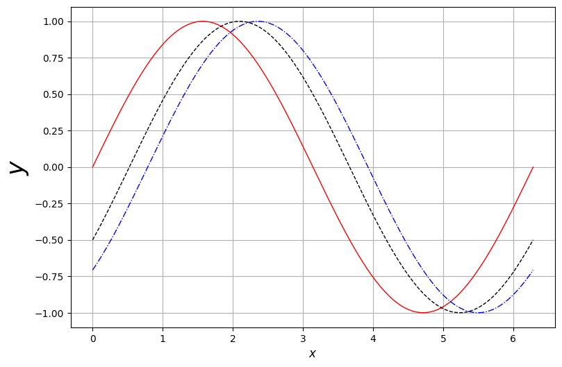

# examples for histogram
# set seed
np.random.seed(2718)
sample = pd.DataFrame(norm.rvs(size=int(5e4)))
sample.head(10), sample.tail(10)

(          0
 0  1.722518
 1 -0.626257
 2 -3.533687
 3  0.716898
 4  1.353317
 5  1.603105
 6  0.501179
 7  0.748855
 8 -1.790165
 9  0.533090,
               0
 49990  0.004426
 49991  0.235329
 49992 -0.188821
 49993 -0.183680
 49994  0.475978
 49995 -1.139552
 49996 -0.162364
 49997 -0.355614
 49998 -0.793454
 49999  1.334050)

sample.describe().transpose()
#sample.describe().transpose()

	count	mean	std	min	25%	50%	75%	max
0	50000.0	0.000345	1.002402	-4.568631	-0.675698	0.006211	0.681126	4.001952

# generate random samples from standard normal
sample = pd.DataFrame(norm.rvs(size=int(5e4))) # 1e5 = 10^5, 1e3 = 10^3 = 1000

x = np.linspace(sample.min(), sample.max(), 200)
y = norm.pdf(x)

# histogram by hvplot.hist
#sample.hvplot.hist(bins=50, height=350, width=550, label='histogram') * \
#hv.Curve((x, y*8500)).opts(color='red', line_dash='dashed')

# histogram by seaborn.histplot
# we shall mostly using this module for plotting histograms
plt.figure(figsize=(9, 6))
sns.histplot(sample[0], bins=50, stat='density', kde=True, label='histogram')

#sns.histplot(sample[0], bins=50, color='k', fill=False)
plt.xlabel('$X$', fontsize=12)
plt.title('Histogram', fontsize=18)

# superimpose density of standard normal 
x = np.linspace(sample.min(), sample.max(), 200)
y = norm.pdf(x)
plt.plot(x, y, 'r--', label='normal density')
plt.legend();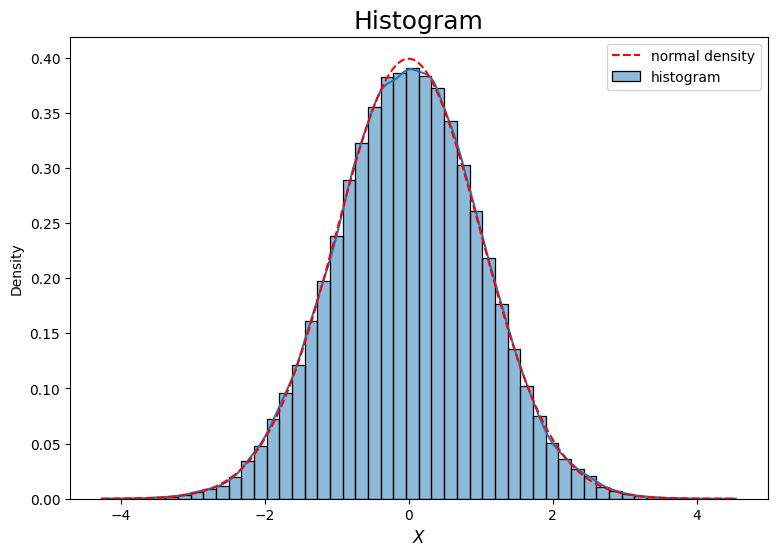

sample.columns = ['X']

# histogram using built-in pandas.DataFrame method
sample.plot(kind='hist', bins=50, density=True, histtype='step')
# superimpose the density
x = np.linspace(sample.min(), sample.max(), 200)
y = norm.pdf(x)
plt.plot(x, y, 'r-.', label='normal density')
plt.xlabel('$X$', fontsize=12)
plt.title('Histogram', fontsize=18)
plt.legend();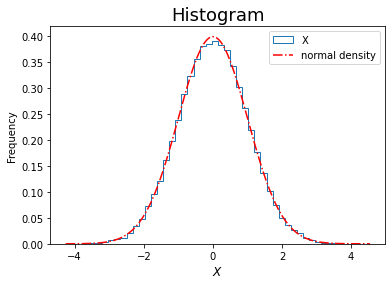

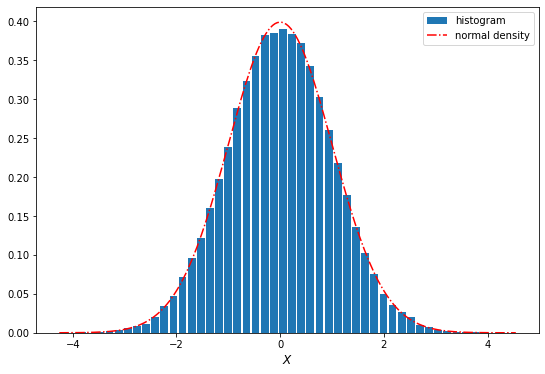
# histogram using pyplot
plt.figure(figsize=(9, 6))
plt.hist(sample, density=True, bins=50, histtype='bar', rwidth=0.85, label='histogram')

# superimpose the density
x = np.linspace(sample.min(), sample.max(), 200)
y = norm.pdf(x)
plt.plot(x, y, 'r-.', label='normal density')
plt.xlabel('$X$', fontsize=12)
plt.legend();

Lecture 1: Financial engineering in a nutshell

Coordinates

Teaching Assistants

Aims of this course

Agenda

Online resources

Financial market

Financial products

What is financial engineering?

What is financial engineering for?

What skills are required to be a financial engineer?

Quantitative analyst - Quant

\(\mathbb{P}\) quant v.s. \(\mathbb{Q}\) quant

Note

Theory of asset pricing

Note

Law of one price

Monotonicity

Linearity

Note

Principle of no arbitrage

Arbitrage opportunity

Fundamental theorem of asset pricing

The First Fundamental Theorem of Asset Pricing

The Second Fundamental Theorem of Asset Pricing

Decentralized Finance (DeFi)

What is DeFi ?

How does DeFi work?

Decentralized Finance Uses

Automated Market Making

Automatic Market Makers (AMMs) are

How AMMs Work

AMM vs CLOB

AMM vs CLOB

Brief introduction to Jupyter notebook and Python

Head 1

Head 2

Head 3

Head 4

numpy.arange vs numpy.linspace

Probability distributions in scipy.stats

`numpy.arange` vs `numpy.linspace`

Probability distributions in `scipy.stats`