Topics in Quantitative Finance, Summer 2025

Lecture 5: Volatility and volatility-linked derivatives

Tai-Ho Wang (王太和)

\[ \newcommand{\bea}{\begin{eqnarray}} \newcommand{\eea}{\end{eqnarray}} \newcommand{\supp}{\mathrm{supp}} \newcommand{\F}{\mathcal{F} } \newcommand{\cF}{\mathcal{F} } \newcommand{\E}{\mathbb{E} } \newcommand{\Eof}[1]{\mathbb{E}\left[ #1 \right]} \newcommand{\Etof}[1]{\mathbb{E}_t\left[ #1 \right]} \def\Cov{{ \text{Cov} }} \def\ES{{ \text{ES} }} \def\Var{{ \text{Var} }} \def\VaR{{ \text{VaR} }} \def\sd{{ \text{sd} }} \def\corr{{ \text{corr} }} \newcommand{\1}{\mathbf{1} } \newcommand{\p}{\partial} \newcommand{\PP}{\mathbb{P} } \newcommand{\Pof}[1]{\mathbb{P}\left[ #1 \right]} \newcommand{\QQ}{\mathbb{Q} } \renewcommand{\R}{\mathbb{R} } \newcommand{\DD}{\mathbb{D} } \newcommand{\HH}{\mathbb{H} } \newcommand{\spn}{\mathrm{span} } \newcommand{\cov}{\mathrm{cov} } \newcommand{\HS}{\mathcal{L}_{\mathrm{HS}} } \newcommand{\Hess}{\mathrm{Hess} } \newcommand{\trace}{\mathrm{trace} } \newcommand{\LL}{\mathcal{L} } \newcommand{\s}{\mathcal{S} } \newcommand{\ee}{\mathcal{E} } \newcommand{\ff}{\mathcal{F} } \newcommand{\hh}{\mathcal{H} } \newcommand{\bb}{\mathcal{B} } \newcommand{\dd}{\mathcal{D} } \newcommand{\g}{\mathcal{G} } \newcommand{\half}{\frac{1}{2} } \newcommand{\T}{\mathcal{T} } \newcommand{\bit}{\begin{itemize}} \newcommand{\eit}{\end{itemize}} \newcommand{\beq}{\begin{equation}} \newcommand{\eeq}{\end{equation}} \newcommand{\tr}{\text{tr}} \renewcommand{\angl}[1]{\langle #1 \rangle} \]

Agenda

Volatility and its various estimators
- Historical volatility
- Implied volatility
- Realized variance
- VIX
Implied volatility
- Estimating discount factor and dividend rates by put-call parity
- GPR fit of implied volatilities
Volatility indices published by CBOE
Volatility linked derivatives
- VIX option
Appendix (Optional)
- Realized variance from high frequency data
- The Corsi HAR-RV forecast

What is volatility?

From the Wikipage:

In finance, volatility (symbol $\sigma$) is the degree of variation of a trading price series over time as measured by the standard deviation of logarithmic returns.

Historic volatility measures a time series of past market prices.

Implied volatility looks forward in time, being derived from the market price of a market-traded derivative (in particular, an option).

Realized variance estimates the integrated variance or quadratic variation by using high frequency data.

注: 波动率是金融资产价格的波动程度.

Why is volatility important?

From the same Wikipage:

Investors care about volatility for at least the following reasons:

The wider the swings in an investment’s price, the harder emotionally it is to not worry;

Price volatility of a trading instrument can define position sizing in a portfolio;

When certain cash flows from selling a security are needed at a specific future date, higher volatility means a greater chance of a shortfall;

Higher volatility of returns while saving for retirement results in a wider distribution of possible final portfolio values;

Higher volatility of return when retired gives withdrawals a larger permanent impact on the portfolio’s value;

Price volatility presents opportunities to buy assets cheaply and sell when overpriced;

Portfolio volatility has a negative impact on the compound annual growth rate (CAGR) of that portfolio

Volatility affects pricing of options, being a parameter of the Black–Scholes model.

In today’s markets, it is also possible to trade volatility directly, through the use of derivative securities such as options and variance swaps.

Volatilities

Volatility of a financial asset in its most preliminary form is defined as the (conditional) standard deviation of its log return. In practice, there exist various notions of “volatility” that are commonly used including

Historical volatility (历史波动率)
Realized and integrated variance/volatility (实际波动率, 一个理论上的, 无法被计算的值)
Implied volatility (隐含波动率, 隐含波动率是制期权市场投资者在进行期权交易时对实际波动率的认识)
Instantaneous volatility (瞬时波动率)

and methods of inferring these volatilities respectively from

Daily or high-frequency time series data of the underlying
Price series of variance swap
Prices of liquidly traded vanilla options

Daily closing prices $S_t$: $S_0, S_1, S_2, ..., S_T$.

Log return $\displaystyle r_t = \log (S_t/S_{t-1})$.

Then the daily volatility is defined as: \[ \sigma_t = \sqrt{\Eof{r_t^2}} = \sqrt{\Eof{\left(\log S_t/S_{t-1}\right)^2}}. \]

And the annualized volatility is defined as: \[ \sigma_t^{\text{annualized}} = \sqrt{252} \cdot \sigma_t. \]

The constant $\sqrt{252}$ is used to convert the daily volatility to annualized volatility, assuming there are 252 trading days in a year.

Historical volatility

Historical volatility uses, say daily, price series to calculate the sample conditional standard deviation of log returns in rolling time windows of a prespecified width.

Example of historical volatility

Now let’s calculate the volatility of S&P500 using 25-day rolling time windows.

One can calculate the volatility series of the input price series $S_t$, $1 \leq t \leq T$, by the following formula

\[ \sigma_t = \sqrt{\frac N{n-2}\sum_{i=1}^{n-1} (r_i - \bar r)^2}, \quad \text{ for } n \leq t \leq T, \]

where

\[\begin{aligned} r_i &= \ln S_{t + i} - \ln S_{t + i - 1}, \quad \text{for } 1 \leq i \leq n - 1, \\ \bar{r} &= \frac{1}{n-1} \sum_{i=1}^{n-1} r_i. \end{aligned}\]

Note

$n$ denotes the width (number of days) of rolling window
$N$ denotes the number of days in a year, thus $\sqrt N$ is the annualized factor
The first $n-1$ points in the output volatility series appear as NA, for an obvious reason.

Exponentially weighted moving average (EWMA)

An alternative to calculate historical volatility is the exponentially weighted moving average method.

\[ \sigma_t = \sqrt{N(1 - \lambda)\sum_{i=1}^{\infty} \lambda^i (r_{t - i} - \bar r)^2}, \quad \text{ for } n \leq t \leq T, \]

for some $\lambda \in (0, 1)$.

Now let’s dirty our hands …

注: SPX stands for S&P 500 index, which is a stock market index that measures the stock performance of 500 large companies listed on stock exchanges in the United States.

#pip install yfinance

import yfinance as yf

import numpy as np
from numpy import exp, log, sqrt
import scipy.stats as ss
from scipy.stats import norm
import pandas as pd
import yfinance as yf
import matplotlib.pyplot as plt
import statsmodels.formula.api as sm

Tips: You may skip the next 5 cells if you encounter an error.

import os
proxy = 'http://127.0.0.1:7897'
os.environ['HTTP_PROXY'] = proxy
os.environ['HTTPS_PROXY'] = proxy

start, end = '2019-01-01', '2024-07-24'
# download SPX from yahoo finance
spx = yf.Ticker("^GSPC").history(start=start, end=end)

# brief look at the data
spx.info(), spx.isna().sum()

<class 'pandas.core.frame.DataFrame'>
DatetimeIndex: 1398 entries, 2019-01-02 00:00:00-05:00 to 2024-07-23 00:00:00-04:00
Data columns (total 7 columns):
 #   Column        Non-Null Count  Dtype  
---  ------        --------------  -----  
 0   Open          1398 non-null   float64
 1   High          1398 non-null   float64
 2   Low           1398 non-null   float64
 3   Close         1398 non-null   float64
 4   Volume        1398 non-null   int64  
 5   Dividends     1398 non-null   float64
 6   Stock Splits  1398 non-null   float64
dtypes: float64(6), int64(1)
memory usage: 87.4 KB

(None,
 Open            0
 High            0
 Low             0
 Close           0
 Volume          0
 Dividends       0
 Stock Splits    0
 dtype: int64)

# first and last few rows of the data
spx

	Open	High	Low	Close	Volume	Dividends	Stock Splits
Date
2019-01-02 00:00:00-05:00	2476.959961	2519.489990	2467.469971	2510.030029	3733160000	0.0	0.0
2019-01-03 00:00:00-05:00	2491.919922	2493.139893	2443.959961	2447.889893	3858830000	0.0	0.0
2019-01-04 00:00:00-05:00	2474.330078	2538.070068	2474.330078	2531.939941	4234140000	0.0	0.0
2019-01-07 00:00:00-05:00	2535.610107	2566.159912	2524.560059	2549.689941	4133120000	0.0	0.0
2019-01-08 00:00:00-05:00	2568.110107	2579.820068	2547.560059	2574.409912	4120060000	0.0	0.0
...	...	...	...	...	...	...	...
2024-07-17 00:00:00-04:00	5610.069824	5622.490234	5584.810059	5588.270020	4246450000	0.0	0.0
2024-07-18 00:00:00-04:00	5608.560059	5614.049805	5522.810059	5544.589844	4007510000	0.0	0.0
2024-07-19 00:00:00-04:00	5543.370117	5557.500000	5497.040039	5505.000000	3760570000	0.0	0.0
2024-07-22 00:00:00-04:00	5544.540039	5570.359863	5529.040039	5564.410156	3375180000	0.0	0.0
2024-07-23 00:00:00-04:00	5565.299805	5585.339844	5550.899902	5555.740234	3500210000	0.0	0.0

1398 rows × 7 columns

# save data, just in case
# spx.to_csv('spx_07252022.csv')

You may start from here.

# load saved data
spx = pd.read_csv('spx_07252022.csv')
spx.index = spx['Date']
spx = spx.drop('Date', axis=1)

# summary statistics
spx.describe().transpose()

	count	mean	std	min	25%	50%	75%	max
Open	895.0	3.586641e+03	6.613510e+02	2290.709961	2.980045e+03	3.439380e+03	4.213645e+03	4.804510e+03
High	895.0	3.608340e+03	6.637349e+02	2300.729980	2.991620e+03	3.464860e+03	4.239375e+03	4.818620e+03
Low	895.0	3.562902e+03	6.583530e+02	2191.860107	2.963575e+03	3.419930e+03	4.192340e+03	4.780040e+03
Close	895.0	3.587314e+03	6.608265e+02	2237.399902	2.978570e+03	3.443120e+03	4.209795e+03	4.796560e+03
Adj Close	895.0	3.587314e+03	6.608265e+02	2237.399902	2.978570e+03	3.443120e+03	4.209795e+03	4.796560e+03
Volume	895.0	4.069480e+09	1.168092e+09	0.000000	3.337885e+09	3.778890e+09	4.548675e+09	9.878040e+09

# plot spx adjusted close
plt.figure(figsize=(9, 6))
spx['Close'].plot()
plt.ylabel('SPX', fontsize=12)
plt.grid();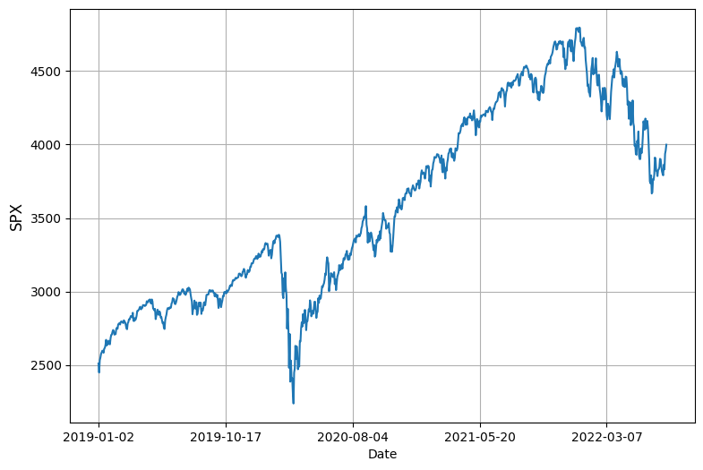

# log return of spx 
r = log(spx['Close']).diff()

# historical volatility in this period
vol = r.std()*sqrt(252)
r, r.mean(), vol, type(r)

(Date
 2019-01-02         NaN
 2019-01-03   -0.025068
 2019-01-04    0.033759
 2019-01-07    0.006986
 2019-01-08    0.009649
                 ...   
 2022-07-15    0.019019
 2022-07-18   -0.008399
 2022-07-19    0.027254
 2022-07-20    0.005878
 2022-07-21    0.009813
 Name: Close, Length: 895, dtype: float64,
 0.0005209587220526575,
 0.22945020327258875,
 pandas.core.series.Series)

# plot log return
plt.figure(figsize=(9, 6))
r.plot(lw=1)
plt.ylabel('SPX log return', fontsize=12)
plt.grid();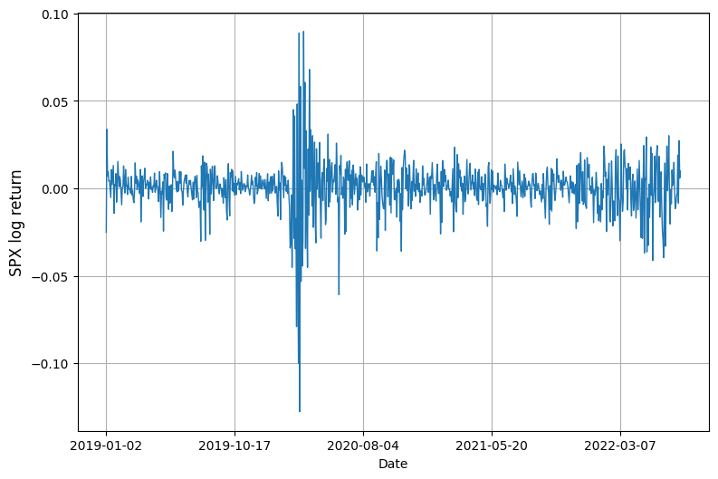

r.iloc[0:10], r.iloc[-10:]

(Date
 2019-01-02         NaN
 2019-01-03   -0.025068
 2019-01-04    0.033759
 2019-01-07    0.006986
 2019-01-08    0.009649
 2019-01-09    0.004090
 2019-01-10    0.004508
 2019-01-11   -0.000146
 2019-01-14   -0.005271
 2019-01-15    0.010665
 Name: Close, dtype: float64,
 Date
 2022-07-08   -0.000831
 2022-07-11   -0.011594
 2022-07-12   -0.009287
 2022-07-13   -0.004467
 2022-07-14   -0.003003
 2022-07-15    0.019019
 2022-07-18   -0.008399
 2022-07-19    0.027254
 2022-07-20    0.005878
 2022-07-21    0.009813
 Name: Close, dtype: float64)

# n: rwidth of rolling window
# N: annualizing factor
def volatility(data, n=10, N=252):
    data = pd.Series(data)
    vol = [np.nan for i in range(n)]
    for i in range(len(data)-n):
        vol += [data.iloc[i:(i+n)].std()*sqrt(N)]
    return pd.DataFrame({'volatility': vol})

volatility(r)

	volatility
0	NaN
1	NaN
2	NaN
3	NaN
4	NaN
...	...
890	0.136786
891	0.160218
892	0.160347
893	0.210679
894	0.211261

895 rows × 1 columns

spx_vol = volatility(r)
spx_vol.index = r.index
plt.figure(figsize=(9, 6))
plt.plot(spx_vol)
plt.ylabel('Volatility', fontsize=12)
plt.title('SPX historical volatility', fontsize=24)
plt.grid();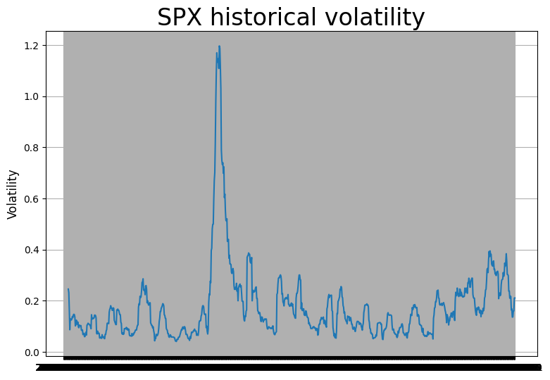

# leverage effect
spx_scaled = (spx - spx.mean())/(spx.max() - spx.min())
plt.figure(figsize=(9, 6))
spx_scaled['Close'].plot(color='k', lw=1, label='scaled spx')
plt.ylim([-0.6, 1])
plt.plot(spx_vol, 'b-.', lw=1, label='volatility')
plt.grid()
plt.title('Leverage effect', fontsize=24)
plt.legend();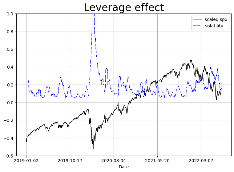

注: Leverage effect (杠杆效应): Stock price 下降, Volatility 上升. Stock price 上升, Volatility 下降.

Equity index returns interact negatively with return volatilities.

Carr, Peter, and Liuren Wu. “Leverage Effect, Volatility Feedback, and Self-Exciting Market Disruptions.” The Journal of Financial and Quantitative Analysis, vol. 52, no. 5, 2017, pp. 2119–56. JSTOR, https://www.jstor.org/stable/26590473. Accessed 28 July 2025.

Volatility estimation using OHLC

Parkison
Garman-Klass
Rogers-Satchell
Yang-Zhang

\[\begin{aligned} \sigma_P^2 &= \frac{1}{4\ln2} \frac{1}{n}\sum_{i=1}^n (\ln H_i - \ln L_i)^2, \\ \sigma_{GK}^2 &= \frac{1}{n} \left\{\sum_{i=1}^n \frac{1}{2}(\ln H_i - \ln L_i)^2 - (2\ln2 - 1)(\ln C_i - \ln O_i)^2 \right\}, \\ \sigma_{RS}^2 &= \frac{1}{n} \sum_{i=1}^n u_i(u_i - c_i) + d_i(d_i - c_i), \\ \sigma_{YZ}^2 &= \sigma_O^2 + w\sigma_C^2 + (1 - w)\sigma_P^2, \quad w = \frac{0.34}{1.34 + \frac{n+1}{n-1}}. \end{aligned}\]

$u_i = \ln H_i - \ln O_i$: daily high weighted by open,
$d_i = \ln L_i - \ln O_i$: daily low weighted by open
$o_i = \ln O_i - \ln C_{i-1}$
$c_i = \ln C_i - \ln O_i$

We make the calculation of these volatilties into a python class.

class Volatilities:
    def __init__(self, OHLC, n=10, N=252):
        self.n = n
        self.N = N
        self.OHLC = pd.DataFrame(OHLC)
        self.o = self.OHLC.Open
        self.h = self.OHLC.High
        self.l = self.OHLC.Low
        self.c = self.OHLC.Close
        self.r = log(self.OHLC['Close']).diff()
        self.vols_c = [np.nan for i in range(self.n)] 
        self.vols_p = [np.nan for i in range(self.n)]
        self.vols_gk = [np.nan for i in range(self.n)] 
        self.vols_rs = [np.nan for i in range(self.n)] 
        
        for i in range(len(self.r) - self.n):
            self.vols_c += [self.r.iloc[i:(i+self.n)].std()*sqrt(self.N)]
            self.vols_p += [self.cal_vol_p(self.h.iloc[i:(i+self.n)], self.l.iloc[i:(i+self.n)])*sqrt(self.N)]
            self.vols_gk += [self.cal_vol_gk(self.o.iloc[i:(i+self.n)], self.h.iloc[i:(i+self.n)], self.l.iloc[i:(i+self.n)], self.c.iloc[i:(i+self.n)])*sqrt(self.N)]
            self.vols_rs += [self.cal_vol_rs(self.o.iloc[i:(i+self.n)], self.h.iloc[i:(i+self.n)], self.l.iloc[i:(i+self.n)], self.c.iloc[i:(i+self.n)])*sqrt(self.N)]
        self.vols = pd.DataFrame({'close': self.vols_c, 'parkinson': self.vols_p, 'garman-klass': self.vols_gk, 'rogers-satchell': self.vols_rs})
        self.vols.index = self.OHLC.index
        
    def cal_vol_p(self, H, L):
        return np.sqrt(((log(H) - log(L))**2).mean()/log(2)/4)
    
    def cal_vol_gk(self, O, H, L, C):
        term1 = ((log(H) - log(L))**2).mean()/2
        term2 = (2*log(2) - 1)*((log(C) - log(O))**2).mean()
        return np.sqrt(term1 - term2)
    
    def cal_vol_rs(self, O, H, L, C):
        u, d, c = log(H) - log(O), log(L) - log(O), log(C) - log(O)
        return np.sqrt((u*(u-c)).mean() + (d*(d-c)).mean())

%%time
spx_vols = Volatilities(spx)

CPU times: total: 344 ms
Wall time: 1.69 s

spx_vols.vols['garman-klass']

Date
2019-01-02         NaN
2019-01-03         NaN
2019-01-04         NaN
2019-01-07         NaN
2019-01-08         NaN
                ...   
2022-07-15    0.128716
2022-07-18    0.126178
2022-07-19    0.138915
2022-07-20    0.140416
2022-07-21    0.140299
Name: garman-klass, Length: 895, dtype: float64

plt.figure(figsize=(10, 6))
spx_vols.vols['close'].plot(ls='--', label='Close', lw=0.8)
spx_vols.vols['parkinson'].plot(lw=0.8, label='Parkinson')
spx_vols.vols['garman-klass'].plot(lw=0.8, label='Garman-Klass')
spx_vols.vols['rogers-satchell'].plot(lw=0.8, label='Rogers-Satchell')
plt.legend()
plt.grid();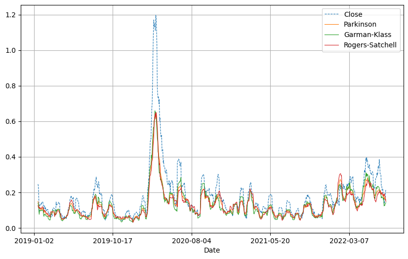

spx.tail(1)

	Open	High	Low	Close	Adj Close	Volume
Date
2022-07-21	3955.469971	3999.290039	3927.639893	3998.949951	3998.949951	3586030000

Implied volatility

“A wrong number to a wrong formula for a correct answer.”

注: wrong number = volatility, wrong formula = Black-Scholes formula, correct answer = option price.

In the Black-Scholes model there is a one-to-one relation between the price of the option and the volatility parameter $\sigma$. The option prices are often quoted by stating this specific volatility, called the implied volatility.
In Black-Scholes world, the volatility is assumed constant. But in reality, options of different strike require different volatilities to match their market prices. This is called the volatility smile.
Most of the work was inspired in modeling the implied volatility.

Why implied volatility rather than the price itself?

Price of a call option is decreasing in strike and increasing in time to expiry
Price of a far out-of-money option is small whereas price of a far in-the-money option carries mostly the intrinsic value
Statistically speaking, implied volatility is a more standard quantity to infer
Traders trade options in terms of implied volatilities rather than their prices

注:

期权价格本身不具备标准化, 不同期权之间不能直接比较; 但波动率是一个标准化的参数, 它不依赖 strike 或 expiry, 因此更便于比较.
期权价格的构成不一致, 有的主要是时间价值, 有的主要是内在价值; 隐含波动率剥离了内在价值, 只反映市场对未来波动的预期, 是一个更“干净”的指标.
你可以比较今天和昨天的隐含波动率来判断市场情绪变化; 但比较期权价格则可能受行权价、到期日等因素干扰.

注: 隐含波动率是市场通过期权的价格推导出的一种预期未来波动率, 它不代表过去的价格波动, 而是预测未来的价格波动区间. IV值高, 意味着市场认为未来价格波动较大; IV 值低, 则意味着市场预期未来波动较小.

期权的价格主要由四个因素决定: 标的资产价格、执行价格、到期时间和波动率. 隐含波动率是唯一一个通过市场价格间接估算出来的变量, 因此它在期权交易中的地位尤为特殊.

隐含波动率与期权价格呈正相关关系. 简单来说, IV 越高, 期权价格越高; IV越低, 期权价格越便宜. 这是因为高隐含波动率意味着标的资产未来可能出现较大的价格波动, 买方愿意为此支付更多的期权溢价, 而卖方则要求更高的补偿来承担风险.

隐含波动率没有固定的计算公式, 而是通过反推法, 根据期权定价模型 (如 Black-Scholes 模型) 和期权的市场价格来计算. 在实际交易中, 不同执行价的期权隐含波动率常呈现“微笑”或“倾斜”的形态, 这种现象被称为“波动率微笑 (Volatility Smile)”.

深度虚值期权 (OTM) 和深度实值期权 (ITM) 的 IV 通常较高, 因为这些期权受到极端价格变动的影响更大. 平值期权 (ATM) 的IV较低, 因为它更接近当前市场价格, 波动性风险相对较小.

A practical tip for fetching risk free and dividend rates

Q: How to obtain the interest rate $r$ and dividend rate $d$ for the calculation of implied volatility?

A: Put-call parity.

Recall the Put-Call Parity for European options

\[ C - P = Se^{-dT} - K e^{-rT} = e^{-rT} (F - K), \]

where $F$ denotes the forward price of the underlying. Hence, if we regress $C - P$ against $K$, the (negative) slope gives us the discount factor and the intercept gives the ex-dividend underlying.

$F = S e^{-(d-r)T}$, which means we can get the dividend rate $d$ by the intercept $F$.

Example - Implied volatilities of options on SPX

# import required modules
import datetime
from datetime import datetime as dt
import numpy as np
from numpy import exp, log, sqrt
import scipy.stats as ss
from scipy.stats import norm
import pandas as pd
import yfinance as yf
import matplotlib.pyplot as plt
import statsmodels.formula.api as sm

Tips: You may skip the next 12 cells if you encounter an error.

# download spx options data from yahoo finance
spx = yf.Ticker('^SPX')
spx_expiries = spx.options
print(spx_expiries)

('2025-07-28', '2025-07-29', '2025-07-30', '2025-07-31', '2025-08-01', '2025-08-04', '2025-08-05', '2025-08-06', '2025-08-07', '2025-08-08', '2025-08-11', '2025-08-12', '2025-08-13', '2025-08-14', '2025-08-15', '2025-08-18', '2025-08-19', '2025-08-20', '2025-08-21', '2025-08-22', '2025-08-25', '2025-08-26', '2025-08-27', '2025-08-28', '2025-08-29', '2025-09-02', '2025-09-05', '2025-09-08', '2025-09-12', '2025-09-19', '2025-09-30', '2025-10-17', '2025-10-31', '2025-11-21', '2025-11-28', '2025-12-19', '2025-12-31', '2026-01-16', '2026-02-20', '2026-03-20', '2026-03-31', '2026-04-17', '2026-05-15', '2026-06-18', '2026-06-30', '2026-07-17', '2026-08-21', '2026-09-18', '2026-12-18', '2027-06-17', '2027-12-17', '2028-12-15', '2029-12-21', '2030-12-20')

# choose an expiry 
idx = 17
today = dt.strftime(dt.now(), '%Y-%m-%d')
day_count = (dt.strptime(spx_expiries[idx], '%Y-%m-%d') - dt.now()).days
print(f'option expiry = {spx_expiries[idx]}, today = {today}')
print(f'There are {day_count} days to expiry')
option_chain = spx.option_chain(spx_expiries[idx])
spx_calls = option_chain.calls
spx_puts = option_chain.puts

option expiry = 2025-08-20, today = 2025-07-28
There are 22 days to expiry

spx_calls.shape, spx_puts.shape

((55, 14), (84, 14))

spx_calls.info()

<class 'pandas.core.frame.DataFrame'>
RangeIndex: 55 entries, 0 to 54
Data columns (total 14 columns):
 #   Column             Non-Null Count  Dtype              
---  ------             --------------  -----              
 0   contractSymbol     55 non-null     object             
 1   lastTradeDate      55 non-null     datetime64[ns, UTC]
 2   strike             55 non-null     float64            
 3   lastPrice          55 non-null     float64            
 4   bid                55 non-null     float64            
 5   ask                55 non-null     float64            
 6   change             55 non-null     float64            
 7   percentChange      55 non-null     float64            
 8   volume             38 non-null     float64            
 9   openInterest       55 non-null     int64              
 10  impliedVolatility  55 non-null     float64            
 11  inTheMoney         55 non-null     bool               
 12  contractSize       55 non-null     object             
 13  currency           55 non-null     object             
dtypes: bool(1), datetime64[ns, UTC](1), float64(8), int64(1), object(3)
memory usage: 5.8+ KB

spx_calls.isna().sum()

contractSymbol        0
lastTradeDate         0
strike                0
lastPrice             0
bid                   0
ask                   0
change                0
percentChange         0
volume               17
openInterest          0
impliedVolatility     0
inTheMoney            0
contractSize          0
currency              0
dtype: int64

spx_puts.isna().sum()

contractSymbol        0
lastTradeDate         0
strike                0
lastPrice             0
bid                   0
ask                   0
change                0
percentChange         0
volume               19
openInterest          0
impliedVolatility     0
inTheMoney            0
contractSize          0
currency              0
dtype: int64

spx_calls

	contractSymbol	lastTradeDate	strike	lastPrice	bid	ask	volume	impliedVolatility	inTheMoney	contractSize	currency
0	SPXW250820C05100000	2025-07-15 20:12:00+00:00	5100.0	1160.00	1327.3	1335.80	NaN	0.667568	True	REGULAR	USD
1	SPXW250820C05200000	2025-07-16 13:33:29+00:00	5200.0	1080.00	1227.8	1236.30	NaN	0.625065	True	REGULAR	USD
2	SPXW250820C05450000	2025-07-17 18:35:24+00:00	5450.0	873.00	979.4	987.90	NaN	0.520505	True	REGULAR	USD
3	SPXW250820C05600000	2025-07-17 18:39:43+00:00	5600.0	725.75	830.6	839.10	NaN	0.471059	True	REGULAR	USD
4	SPXW250820C06000000	2025-07-25 19:40:13+00:00	6000.0	419.54	438.2	446.60	1.0	0.305007	True	REGULAR	USD
5	SPXW250820C06100000	2025-07-22 19:07:15+00:00	6100.0	263.17	342.9	351.70	NaN	0.265789	True	REGULAR	USD
6	SPXW250820C06150000	2025-07-24 17:14:10+00:00	6150.0	267.38	296.7	305.40	2.0	0.246815	True	REGULAR	USD
7	SPXW250820C06175000	2025-07-14 18:00:54+00:00	6175.0	186.31	273.7	282.50	NaN	0.237251	True	REGULAR	USD
8	SPXW250820C06200000	2025-07-25 19:53:07+00:00	6200.0	232.41	251.6	260.00	33.0	0.227989	True	REGULAR	USD
9	SPXW250820C06225000	2025-07-15 15:00:23+00:00	6225.0	147.87	228.9	237.90	NaN	0.218937	True	REGULAR	USD
10	SPXW250820C06240000	2025-07-22 14:09:40+00:00	6240.0	141.65	215.9	224.80	NaN	0.213516	True	REGULAR	USD
11	SPXW250820C06250000	2025-07-25 19:53:07+00:00	6250.0	189.71	210.5	213.40	33.0	0.205288	True	REGULAR	USD
12	SPXW250820C06260000	2025-07-24 14:14:35+00:00	6260.0	164.55	202.2	204.80	NaN	0.201723	True	REGULAR	USD
13	SPXW250820C06270000	2025-07-24 14:14:35+00:00	6270.0	156.70	193.7	196.30	NaN	0.198216	True	REGULAR	USD
14	SPXW250820C06275000	2025-07-23 19:48:30+00:00	6275.0	147.30	189.2	192.10	6.0	0.196499	True	REGULAR	USD
15	SPXW250820C06280000	2025-07-23 17:30:30+00:00	6280.0	135.77	185.2	187.90	26.0	0.194756	True	REGULAR	USD
16	SPXW250820C06290000	2025-07-24 13:43:32+00:00	6290.0	141.60	176.7	179.60	1.0	0.191334	True	REGULAR	USD
17	SPXW250820C06300000	2025-07-25 19:03:56+00:00	6300.0	151.55	168.5	171.40	4.0	0.187943	True	REGULAR	USD
18	SPXW250820C06310000	2025-07-25 19:03:56+00:00	6310.0	143.79	160.4	163.30	1.0	0.184575	True	REGULAR	USD
19	SPXW250820C06320000	2025-07-25 19:51:42+00:00	6320.0	134.47	153.4	154.20	1.0	0.179478	True	REGULAR	USD
20	SPXW250820C06325000	2025-07-25 19:51:42+00:00	6325.0	130.77	149.4	150.30	5.0	0.177907	True	REGULAR	USD
21	SPXW250820C06330000	2025-07-24 14:25:27+00:00	6330.0	114.00	145.6	146.40	40.0	0.176297	True	REGULAR	USD
22	SPXW250820C06340000	2025-07-25 19:22:20+00:00	6340.0	123.00	137.8	138.70	40.0	0.173102	True	REGULAR	USD
23	SPXW250820C06350000	2025-07-25 18:13:34+00:00	6350.0	114.81	130.2	131.10	15.0	0.169888	True	REGULAR	USD
24	SPXW250820C06360000	2025-07-23 16:41:48+00:00	6360.0	82.10	122.8	123.60	2.0	0.166646	True	REGULAR	USD
25	SPXW250820C06370000	2025-07-25 12:56:28+00:00	6370.0	89.09	115.6	116.40	1.0	0.163667	True	REGULAR	USD
26	SPXW250820C06375000	2025-07-25 14:56:57+00:00	6375.0	87.15	112.0	112.90	4.0	0.162251	True	REGULAR	USD
27	SPXW250820C06380000	2025-07-25 16:19:30+00:00	6380.0	87.71	108.5	109.40	80.0	0.160785	True	REGULAR	USD
28	SPXW250820C06400000	2025-07-25 19:59:21+00:00	6400.0	79.20	94.9	95.80	2.0	0.154961	False	REGULAR	USD
29	SPXW250820C06410000	2025-07-25 15:48:10+00:00	6410.0	67.17	88.4	89.30	1.0	0.152150	False	REGULAR	USD
30	SPXW250820C06420000	2025-07-25 15:11:55+00:00	6420.0	62.95	82.2	83.10	36.0	0.149537	False	REGULAR	USD
31	SPXW250820C06425000	2025-07-25 16:09:42+00:00	6425.0	60.34	79.2	80.10	11.0	0.148286	False	REGULAR	USD
32	SPXW250820C06430000	2025-07-25 15:11:50+00:00	6430.0	57.88	76.2	77.10	18.0	0.146964	False	REGULAR	USD
33	SPXW250820C06440000	2025-07-25 16:22:59+00:00	6440.0	54.59	70.5	71.30	4.0	0.144416	False	REGULAR	USD
34	SPXW250820C06450000	2025-07-25 17:04:55+00:00	6450.0	52.55	65.1	65.90	39.0	0.142198	False	REGULAR	USD
35	SPXW250820C06460000	2025-07-25 19:52:19+00:00	6460.0	49.20	59.8	60.60	3.0	0.139829	False	REGULAR	USD
36	SPXW250820C06470000	2025-07-25 15:29:27+00:00	6470.0	40.74	54.9	55.70	5.0	0.137780	False	REGULAR	USD
37	SPXW250820C06475000	2025-07-25 18:47:39+00:00	6475.0	45.30	52.4	53.30	71.0	0.136712	False	REGULAR	USD
38	SPXW250820C06480000	2025-07-24 14:44:53+00:00	6480.0	37.38	50.2	51.00	NaN	0.135726	False	REGULAR	USD
39	SPXW250820C06500000	2025-07-25 17:56:19+00:00	6500.0	34.52	41.7	42.40	7.0	0.131917	False	REGULAR	USD
40	SPXW250820C06525000	2025-07-25 19:52:20+00:00	6525.0	26.10	32.5	33.10	50.0	0.127639	False	REGULAR	USD
41	SPXW250820C06550000	2025-07-25 19:52:20+00:00	6550.0	19.80	24.9	25.50	14.0	0.124173	False	REGULAR	USD
42	SPXW250820C06575000	2025-07-24 14:22:05+00:00	6575.0	13.00	18.7	19.30	NaN	0.121156	False	REGULAR	USD
43	SPXW250820C06600000	2025-07-25 13:30:56+00:00	6600.0	9.30	13.9	14.50	1.0	0.118940	False	REGULAR	USD
44	SPXW250820C06625000	2025-07-25 17:38:33+00:00	6625.0	8.40	10.1	10.70	5.0	0.116964	False	REGULAR	USD
45	SPXW250820C06650000	2025-07-25 14:10:48+00:00	6650.0	5.00	7.3	7.70	4.0	0.114999	False	REGULAR	USD
46	SPXW250820C06675000	2025-07-25 19:43:31+00:00	6675.0	4.20	5.1	5.60	2.0	0.114015	False	REGULAR	USD
47	SPXW250820C06700000	2025-07-25 14:40:39+00:00	6700.0	2.70	3.6	4.10	5.0	0.113641	False	REGULAR	USD
48	SPXW250820C06725000	2025-07-22 13:37:28+00:00	6725.0	1.97	2.6	2.95	NaN	0.113229	False	REGULAR	USD
49	SPXW250820C06750000	2025-07-23 15:22:01+00:00	6750.0	1.30	1.9	2.15	NaN	0.113351	False	REGULAR	USD
50	SPXW250820C06800000	2025-07-23 14:06:32+00:00	6800.0	0.82	0.0	1.30	1.0	0.116311	False	REGULAR	USD
51	SPXW250820C06900000	2025-07-23 15:47:26+00:00	6900.0	0.45	0.0	0.00	6.0	0.062509	False	REGULAR	USD
52	SPXW250820C07000000	2025-07-23 14:52:42+00:00	7000.0	0.25	0.0	0.00	NaN	0.062509	False	REGULAR	USD
53	SPXW250820C07200000	2025-07-24 13:48:48+00:00	7200.0	0.25	0.0	0.00	NaN	0.062509	False	REGULAR	USD
54	SPXW250820C08000000	2025-07-23 13:30:06+00:00	8000.0	0.05	0.0	0.00	NaN	0.125009	False	REGULAR	USD

# clean up data
# remove NA's
spx_calls = spx_calls.drop(['currency', 'contractSize'], axis=1).dropna()
spx_puts = spx_puts.drop(['currency', 'contractSize'], axis=1).dropna()
spx_calls.shape, spx_puts.shape

((38, 12), (65, 12))

spx_calls[spx_calls['lastTradeDate'] > '2024-07']

	contractSymbol	lastTradeDate	strike	lastPrice	bid	ask	volume	impliedVolatility	inTheMoney
4	SPXW250820C06000000	2025-07-25 19:40:13+00:00	6000.0	419.54	438.2	446.6	1.0	0.305007	True
6	SPXW250820C06150000	2025-07-24 17:14:10+00:00	6150.0	267.38	296.7	305.4	2.0	0.246815	True
8	SPXW250820C06200000	2025-07-25 19:53:07+00:00	6200.0	232.41	251.6	260.0	33.0	0.227989	True
11	SPXW250820C06250000	2025-07-25 19:53:07+00:00	6250.0	189.71	210.5	213.4	33.0	0.205288	True
14	SPXW250820C06275000	2025-07-23 19:48:30+00:00	6275.0	147.30	189.2	192.1	6.0	0.196499	True
15	SPXW250820C06280000	2025-07-23 17:30:30+00:00	6280.0	135.77	185.2	187.9	26.0	0.194756	True
16	SPXW250820C06290000	2025-07-24 13:43:32+00:00	6290.0	141.60	176.7	179.6	1.0	0.191334	True
17	SPXW250820C06300000	2025-07-25 19:03:56+00:00	6300.0	151.55	168.5	171.4	4.0	0.187943	True
18	SPXW250820C06310000	2025-07-25 19:03:56+00:00	6310.0	143.79	160.4	163.3	1.0	0.184575	True
19	SPXW250820C06320000	2025-07-25 19:51:42+00:00	6320.0	134.47	153.4	154.2	1.0	0.179478	True
20	SPXW250820C06325000	2025-07-25 19:51:42+00:00	6325.0	130.77	149.4	150.3	5.0	0.177907	True
21	SPXW250820C06330000	2025-07-24 14:25:27+00:00	6330.0	114.00	145.6	146.4	40.0	0.176297	True
22	SPXW250820C06340000	2025-07-25 19:22:20+00:00	6340.0	123.00	137.8	138.7	40.0	0.173102	True
23	SPXW250820C06350000	2025-07-25 18:13:34+00:00	6350.0	114.81	130.2	131.1	15.0	0.169888	True
24	SPXW250820C06360000	2025-07-23 16:41:48+00:00	6360.0	82.10	122.8	123.6	2.0	0.166646	True
25	SPXW250820C06370000	2025-07-25 12:56:28+00:00	6370.0	89.09	115.6	116.4	1.0	0.163667	True
26	SPXW250820C06375000	2025-07-25 14:56:57+00:00	6375.0	87.15	112.0	112.9	4.0	0.162251	True
27	SPXW250820C06380000	2025-07-25 16:19:30+00:00	6380.0	87.71	108.5	109.4	80.0	0.160785	True
28	SPXW250820C06400000	2025-07-25 19:59:21+00:00	6400.0	79.20	94.9	95.8	2.0	0.154961	False
29	SPXW250820C06410000	2025-07-25 15:48:10+00:00	6410.0	67.17	88.4	89.3	1.0	0.152150	False
30	SPXW250820C06420000	2025-07-25 15:11:55+00:00	6420.0	62.95	82.2	83.1	36.0	0.149537	False
31	SPXW250820C06425000	2025-07-25 16:09:42+00:00	6425.0	60.34	79.2	80.1	11.0	0.148286	False
32	SPXW250820C06430000	2025-07-25 15:11:50+00:00	6430.0	57.88	76.2	77.1	18.0	0.146964	False
33	SPXW250820C06440000	2025-07-25 16:22:59+00:00	6440.0	54.59	70.5	71.3	4.0	0.144416	False
34	SPXW250820C06450000	2025-07-25 17:04:55+00:00	6450.0	52.55	65.1	65.9	39.0	0.142198	False
35	SPXW250820C06460000	2025-07-25 19:52:19+00:00	6460.0	49.20	59.8	60.6	3.0	0.139829	False
36	SPXW250820C06470000	2025-07-25 15:29:27+00:00	6470.0	40.74	54.9	55.7	5.0	0.137780	False
37	SPXW250820C06475000	2025-07-25 18:47:39+00:00	6475.0	45.30	52.4	53.3	71.0	0.136712	False
39	SPXW250820C06500000	2025-07-25 17:56:19+00:00	6500.0	34.52	41.7	42.4	7.0	0.131917	False
40	SPXW250820C06525000	2025-07-25 19:52:20+00:00	6525.0	26.10	32.5	33.1	50.0	0.127639	False
41	SPXW250820C06550000	2025-07-25 19:52:20+00:00	6550.0	19.80	24.9	25.5	14.0	0.124173	False
43	SPXW250820C06600000	2025-07-25 13:30:56+00:00	6600.0	9.30	13.9	14.5	1.0	0.118940	False
44	SPXW250820C06625000	2025-07-25 17:38:33+00:00	6625.0	8.40	10.1	10.7	5.0	0.116964	False
45	SPXW250820C06650000	2025-07-25 14:10:48+00:00	6650.0	5.00	7.3	7.7	4.0	0.114999	False
46	SPXW250820C06675000	2025-07-25 19:43:31+00:00	6675.0	4.20	5.1	5.6	2.0	0.114015	False
47	SPXW250820C06700000	2025-07-25 14:40:39+00:00	6700.0	2.70	3.6	4.1	5.0	0.113641	False
50	SPXW250820C06800000	2025-07-23 14:06:32+00:00	6800.0	0.82	0.0	1.3	1.0	0.116311	False
51	SPXW250820C06900000	2025-07-23 15:47:26+00:00	6900.0	0.45	0.0	0.0	6.0	0.062509	False

# remove data point where either bid = 0 or ask = 0
# remove data that that are not traded recently
spx_calls = spx_calls[(spx_calls['bid'] > 0) & (spx_calls['ask'] > 0)]
#spx_calls[spx_calls['lastTradeDate'] > '2022-07']
spx_calls

	contractSymbol	lastTradeDate	strike	lastPrice	bid	ask	volume	impliedVolatility	inTheMoney
4	SPXW250820C06000000	2025-07-25 19:40:13+00:00	6000.0	419.54	438.2	446.6	1.0	0.305007	True
6	SPXW250820C06150000	2025-07-24 17:14:10+00:00	6150.0	267.38	296.7	305.4	2.0	0.246815	True
8	SPXW250820C06200000	2025-07-25 19:53:07+00:00	6200.0	232.41	251.6	260.0	33.0	0.227989	True
11	SPXW250820C06250000	2025-07-25 19:53:07+00:00	6250.0	189.71	210.5	213.4	33.0	0.205288	True
14	SPXW250820C06275000	2025-07-23 19:48:30+00:00	6275.0	147.30	189.2	192.1	6.0	0.196499	True
15	SPXW250820C06280000	2025-07-23 17:30:30+00:00	6280.0	135.77	185.2	187.9	26.0	0.194756	True
16	SPXW250820C06290000	2025-07-24 13:43:32+00:00	6290.0	141.60	176.7	179.6	1.0	0.191334	True
17	SPXW250820C06300000	2025-07-25 19:03:56+00:00	6300.0	151.55	168.5	171.4	4.0	0.187943	True
18	SPXW250820C06310000	2025-07-25 19:03:56+00:00	6310.0	143.79	160.4	163.3	1.0	0.184575	True
19	SPXW250820C06320000	2025-07-25 19:51:42+00:00	6320.0	134.47	153.4	154.2	1.0	0.179478	True
20	SPXW250820C06325000	2025-07-25 19:51:42+00:00	6325.0	130.77	149.4	150.3	5.0	0.177907	True
21	SPXW250820C06330000	2025-07-24 14:25:27+00:00	6330.0	114.00	145.6	146.4	40.0	0.176297	True
22	SPXW250820C06340000	2025-07-25 19:22:20+00:00	6340.0	123.00	137.8	138.7	40.0	0.173102	True
23	SPXW250820C06350000	2025-07-25 18:13:34+00:00	6350.0	114.81	130.2	131.1	15.0	0.169888	True
24	SPXW250820C06360000	2025-07-23 16:41:48+00:00	6360.0	82.10	122.8	123.6	2.0	0.166646	True
25	SPXW250820C06370000	2025-07-25 12:56:28+00:00	6370.0	89.09	115.6	116.4	1.0	0.163667	True
26	SPXW250820C06375000	2025-07-25 14:56:57+00:00	6375.0	87.15	112.0	112.9	4.0	0.162251	True
27	SPXW250820C06380000	2025-07-25 16:19:30+00:00	6380.0	87.71	108.5	109.4	80.0	0.160785	True
28	SPXW250820C06400000	2025-07-25 19:59:21+00:00	6400.0	79.20	94.9	95.8	2.0	0.154961	False
29	SPXW250820C06410000	2025-07-25 15:48:10+00:00	6410.0	67.17	88.4	89.3	1.0	0.152150	False
30	SPXW250820C06420000	2025-07-25 15:11:55+00:00	6420.0	62.95	82.2	83.1	36.0	0.149537	False
31	SPXW250820C06425000	2025-07-25 16:09:42+00:00	6425.0	60.34	79.2	80.1	11.0	0.148286	False
32	SPXW250820C06430000	2025-07-25 15:11:50+00:00	6430.0	57.88	76.2	77.1	18.0	0.146964	False
33	SPXW250820C06440000	2025-07-25 16:22:59+00:00	6440.0	54.59	70.5	71.3	4.0	0.144416	False
34	SPXW250820C06450000	2025-07-25 17:04:55+00:00	6450.0	52.55	65.1	65.9	39.0	0.142198	False
35	SPXW250820C06460000	2025-07-25 19:52:19+00:00	6460.0	49.20	59.8	60.6	3.0	0.139829	False
36	SPXW250820C06470000	2025-07-25 15:29:27+00:00	6470.0	40.74	54.9	55.7	5.0	0.137780	False
37	SPXW250820C06475000	2025-07-25 18:47:39+00:00	6475.0	45.30	52.4	53.3	71.0	0.136712	False
39	SPXW250820C06500000	2025-07-25 17:56:19+00:00	6500.0	34.52	41.7	42.4	7.0	0.131917	False
40	SPXW250820C06525000	2025-07-25 19:52:20+00:00	6525.0	26.10	32.5	33.1	50.0	0.127639	False
41	SPXW250820C06550000	2025-07-25 19:52:20+00:00	6550.0	19.80	24.9	25.5	14.0	0.124173	False
43	SPXW250820C06600000	2025-07-25 13:30:56+00:00	6600.0	9.30	13.9	14.5	1.0	0.118940	False
44	SPXW250820C06625000	2025-07-25 17:38:33+00:00	6625.0	8.40	10.1	10.7	5.0	0.116964	False
45	SPXW250820C06650000	2025-07-25 14:10:48+00:00	6650.0	5.00	7.3	7.7	4.0	0.114999	False
46	SPXW250820C06675000	2025-07-25 19:43:31+00:00	6675.0	4.20	5.1	5.6	2.0	0.114015	False
47	SPXW250820C06700000	2025-07-25 14:40:39+00:00	6700.0	2.70	3.6	4.1	5.0	0.113641	False

spx_puts = spx_puts[(spx_puts['bid'] > 0) & (spx_puts['ask'] > 0)]
#spx_puts = spx_puts[spx_puts['lastTradeDate'] > '2022-02']
spx_puts

	contractSymbol	lastTradeDate	strike	lastPrice	bid	ask	change	percentChange	volume	impliedVolatility	inTheMoney
6	SPXW250820P04800000	2025-07-23 19:03:36+00:00	4800.0	1.55	0.70	0.90	0.000000	0.000000	23.0	0.429327	False
11	SPXW250820P05400000	2025-07-25 19:37:03+00:00	5400.0	2.85	2.20	2.40	0.000000	0.000000	1.0	0.301795	False
12	SPXW250820P05425000	2025-07-25 20:02:09+00:00	5425.0	2.80	2.30	2.50	0.000000	0.000000	1590.0	0.296272	False
13	SPXW250820P05450000	2025-07-25 20:00:17+00:00	5450.0	3.00	2.40	2.60	0.000000	0.000000	4.0	0.290657	False
14	SPXW250820P05500000	2025-07-25 20:00:51+00:00	5500.0	3.32	2.65	2.85	0.000000	0.000000	100.0	0.279884	False
17	SPXW250820P05575000	2025-07-21 18:22:57+00:00	5575.0	6.30	3.00	3.30	0.000000	0.000000	25.0	0.263801	False
19	SPXW250820P05625000	2025-07-25 19:45:59+00:00	5625.0	4.30	3.30	3.60	0.000000	0.000000	61.0	0.252449	False
21	SPXW250820P05675000	2025-07-24 19:45:17+00:00	5675.0	5.10	3.70	4.00	0.000000	0.000000	1.0	0.241646	False
22	SPXW250820P05700000	2025-07-24 20:08:32+00:00	5700.0	5.80	3.90	4.20	0.000000	0.000000	23.0	0.236031	False
24	SPXW250820P05750000	2025-07-24 13:54:07+00:00	5750.0	6.00	4.30	4.70	0.000000	0.000000	72.0	0.225182	False
25	SPXW250820P05775000	2025-07-23 18:05:17+00:00	5775.0	7.47	4.60	5.00	0.000000	0.000000	67.0	0.219902	False
26	SPXW250820P05800000	2025-07-24 19:57:36+00:00	5800.0	7.25	4.90	5.30	0.000000	0.000000	807.0	0.214394	False
27	SPXW250820P05825000	2025-07-23 19:59:30+00:00	5825.0	8.40	5.20	5.60	0.000000	0.000000	20.0	0.208702	False
28	SPXW250820P05850000	2025-07-25 19:44:58+00:00	5850.0	7.30	5.60	6.00	0.000000	0.000000	12.0	0.203469	False
29	SPXW250820P05875000	2025-07-25 20:03:13+00:00	5875.0	7.70	6.10	6.40	0.000000	0.000000	41.0	0.197976	False
30	SPXW250820P05900000	2025-07-25 19:03:54+00:00	5900.0	8.20	6.60	6.90	0.000000	0.000000	4.0	0.192833	False
31	SPXW250820P05925000	2025-07-25 15:01:11+00:00	5925.0	9.40	7.10	7.50	0.000000	0.000000	6.0	0.187905	False
32	SPXW250820P05950000	2025-07-25 19:44:10+00:00	5950.0	9.90	7.80	8.10	0.000000	0.000000	12.0	0.182625	False
33	SPXW250820P05975000	2025-07-25 15:29:05+00:00	5975.0	11.16	8.50	8.90	0.000000	0.000000	1.0	0.177949	False
34	SPXW250820P06000000	2025-07-25 19:44:29+00:00	6000.0	12.10	9.40	9.70	0.000000	0.000000	6.0	0.172814	False
35	SPXW250820P06025000	2025-07-23 20:06:00+00:00	6025.0	17.34	10.40	10.70	0.000000	0.000000	2.0	0.168069	False
36	SPXW250820P06050000	2025-07-28 00:15:00+00:00	6050.0	12.18	11.40	11.80	-2.320000	-15.999998	5.0	0.163186	False
37	SPXW250820P06075000	2025-07-28 00:15:00+00:00	6075.0	13.58	12.60	13.10	-2.719999	-16.687113	5.0	0.158463	False
38	SPXW250820P06100000	2025-07-25 18:15:22+00:00	6100.0	18.15	14.10	14.70	0.000000	0.000000	11.0	0.154084	False
39	SPXW250820P06110000	2025-07-25 19:35:59+00:00	6110.0	18.72	14.70	15.20	0.000000	0.000000	4.0	0.151711	False
40	SPXW250820P06125000	2025-07-23 20:06:00+00:00	6125.0	26.39	15.70	16.20	0.000000	0.000000	95.0	0.148728	False
42	SPXW250820P06140000	2025-07-23 14:37:25+00:00	6140.0	36.73	16.80	17.30	0.000000	0.000000	5.0	0.145768	False
43	SPXW250820P06150000	2025-07-25 19:51:42+00:00	6150.0	22.40	17.60	18.10	0.000000	0.000000	33.0	0.143830	False
45	SPXW250820P06170000	2025-07-23 15:57:02+00:00	6170.0	35.67	19.20	19.80	0.000000	0.000000	2.0	0.139833	False
46	SPXW250820P06175000	2025-07-28 00:15:00+00:00	6175.0	20.83	19.70	20.20	-9.469999	-31.254124	2.0	0.138692	False
48	SPXW250820P06190000	2025-07-25 14:54:57+00:00	6190.0	28.37	21.10	21.60	0.000000	0.000000	5.0	0.135568	False
49	SPXW250820P06200000	2025-07-28 00:15:00+00:00	6200.0	23.43	22.10	22.60	-4.570000	-16.321428	2.0	0.133466	False
52	SPXW250820P06225000	2025-07-25 19:52:19+00:00	6225.0	31.30	24.80	25.50	0.000000	0.000000	3.0	0.128450	False
53	SPXW250820P06230000	2025-07-25 19:59:09+00:00	6230.0	32.20	25.40	26.10	0.000000	0.000000	3.0	0.127370	False
55	SPXW250820P06250000	2025-07-25 19:59:02+00:00	6250.0	35.20	27.90	28.50	0.000000	0.000000	12.0	0.122655	False
56	SPXW250820P06260000	2025-07-25 19:59:00+00:00	6260.0	36.80	29.40	29.90	0.000000	0.000000	3.0	0.120439	False
58	SPXW250820P06275000	2025-07-25 18:25:43+00:00	6275.0	39.51	31.60	32.10	0.000000	0.000000	14.0	0.116964	False
59	SPXW250820P06280000	2025-07-25 19:59:05+00:00	6280.0	40.70	32.30	32.90	0.000000	0.000000	8.0	0.115834	False
60	SPXW250820P06290000	2025-07-25 19:59:16+00:00	6290.0	42.80	34.00	34.60	0.000000	0.000000	3.0	0.113599	False
61	SPXW250820P06300000	2025-07-25 20:11:02+00:00	6300.0	44.80	35.70	36.40	0.000000	0.000000	15.0	0.111326	False
62	SPXW250820P06310000	2025-07-25 19:59:42+00:00	6310.0	47.20	37.60	38.30	0.000000	0.000000	4.0	0.108999	False
63	SPXW250820P06320000	2025-07-25 19:35:39+00:00	6320.0	48.85	39.60	40.20	0.000000	0.000000	3.0	0.106435	False
64	SPXW250820P06325000	2025-07-25 13:47:22+00:00	6325.0	57.90	40.60	41.30	0.000000	0.000000	4.0	0.105314	False
65	SPXW250820P06330000	2025-07-25 19:35:56+00:00	6330.0	51.45	41.70	42.30	0.000000	0.000000	7.0	0.103959	False
66	SPXW250820P06340000	2025-07-25 13:37:46+00:00	6340.0	61.92	43.90	44.60	0.000000	0.000000	4.0	0.101545	False
67	SPXW250820P06350000	2025-07-25 19:58:36+00:00	6350.0	57.50	46.30	47.00	0.000000	0.000000	11.0	0.099000	False
68	SPXW250820P06360000	2025-07-25 14:30:50+00:00	6360.0	66.90	48.70	49.50	0.000000	0.000000	1.0	0.096311	False
70	SPXW250820P06375000	2025-07-25 19:52:10+00:00	6375.0	66.77	52.90	53.70	0.000000	0.000000	1.0	0.092359	False
71	SPXW250820P06380000	2025-07-25 19:52:19+00:00	6380.0	67.10	54.40	55.20	0.000000	0.000000	2.0	0.091013	False
72	SPXW250820P06390000	2025-07-25 19:52:19+00:00	6390.0	70.80	57.40	58.20	0.000000	0.000000	3.0	0.088033	True
73	SPXW250820P06400000	2025-07-25 19:52:19+00:00	6400.0	74.70	60.70	61.50	0.000000	0.000000	2.0	0.085088	True
75	SPXW250820P06420000	2025-07-25 19:57:32+00:00	6420.0	83.10	68.00	68.90	0.000000	0.000000	1.0	0.078977	True
76	SPXW250820P06425000	2025-07-25 19:58:28+00:00	6425.0	84.90	69.90	70.80	0.000000	0.000000	1.0	0.077177	True
79	SPXW250820P06450000	2025-07-25 17:59:21+00:00	6450.0	98.02	80.70	81.60	0.000000	0.000000	63.0	0.067556	True
81	SPXW250820P06550000	2025-07-25 19:36:12+00:00	6550.0	162.00	139.50	142.20	0.000000	0.000000	1.0	0.000010	True

# save data as csv
#spx_calls.to_csv('spxcall_07252022.csv', index=False)
#spx_puts.to_csv('spxput_07252022.csv', index=False)

You may start from here

# read saved spx option data
spx_calls = pd.read_csv('spxcall_07252022.csv')
spx_puts = pd.read_csv('spxput_07252022.csv')

Create `python` class `OptionAnalytics`

Wrap everything up in a python class.

class OptionAnalytics:
    def __init__(self, option_chain, expiry, today):
        self.expiry = expiry
        self.today = today
        if not type(today) == datetime.datetime:
            self.today = dt.strptime(today, '%Y-%m-%d')
        self.calls, self.puts = option_chain
        self.ks_c = self.calls['strike']
        self.cs = (self.calls['bid'] + self.calls['ask'])/2 
        self.ks_p = self.puts['strike'] 
        self.ps = (self.puts['bid'] + self.puts['ask'])/2         
        # strikes that are traded for both calls and puts
        self.ks = np.array([])
        for k in self.ks_c:
            if k in np.array(self.ks_p):
                self.ks = np.concatenate([self.ks, [k]])

        self.mids_call = np.array([])
        for k in self.ks:
            self.calls[self.calls['strike'] == k]['bid']
            bid = self.calls[self.calls['strike'] == k]['bid']
            ask = self.calls[self.calls['strike'] == k]['ask']
            self.mids_call = np.concatenate([self.mids_call, np.array((bid + ask)/2)])

        self.mids_put = np.array([])
        for k in self.ks:
            bid = self.puts[self.puts['strike'] == k]['bid']
            ask = self.puts[self.puts['strike'] == k]['ask']
            self.mids_put = np.concatenate([self.mids_put, np.array((bid + ask)/2)])
            
        tmp = self.imp_vols()
        self.ivs, self.s_adj = tmp['imp_vols'], tmp['s_adj']
        
    # put-call parity plot 
    def plot_parity(self):
        plt.figure(figsize=(9, 5))
        plt.plot(self.ks, self.mids_call - self.mids_put, 'r.--')
        plt.ylabel(r'$C - P$', fontsize=12)
        plt.xlabel(r'$K$', fontsize=12)
        plt.title(f'Expiry: {self.expiry}', fontsize=15);
        return None
            
    def plot_arb(self):
        # monotonicity and convexity for option premia vs strikes
        fig, axes = plt.subplots(1, 2, figsize=(12, 5), sharey=True)
        axes[0].plot(self.ks_c, self.cs, 'bo--')
        axes[0].set_ylabel('Option mid price', fontsize=12)
        axes[0].set_xlabel('Strike', fontsize=12)
        axes[1].plot(self.ks_p, self.ps, 'ro--')
        axes[1].set_xlabel('Strike', fontsize=12);
        return None
        
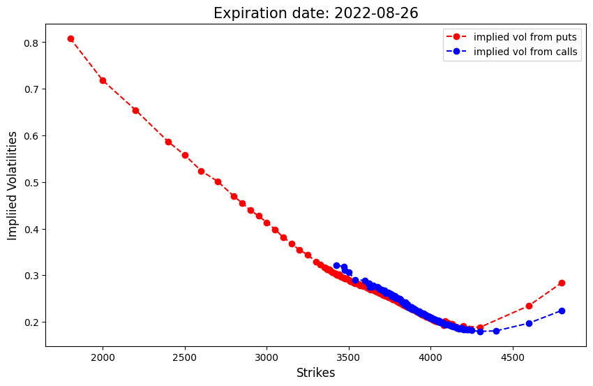
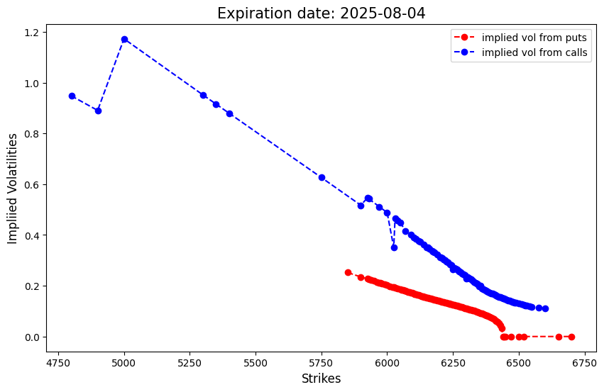
    # plot implied vol
    def plot_imp_vols1(self):
        ivs_c = self.calls['impliedVolatility']
        ivs_p = self.puts['impliedVolatility']
        # plot 
        plt.figure(figsize=(10, 6))
        plt.plot(self.ks_p, ivs_p, 'ro--', label='implied vol from puts')
        plt.plot(self.ks_c, ivs_c, 'bo--', label='implied vol from calls')
        plt.title(f'Expiration date: {self.expiry}', fontsize=15)
        plt.xlabel('Strikes', fontsize=12)
        plt.ylabel('Impliied Volatilities', fontsize=12)
        plt.legend();
        return None
        
    # Black-Scholes formula for call
    def bs_call(self, s, K, t, sigma, r=0):
        d1 = (log(s/K) + r*t)/(sigma*sqrt(t)) + sigma*sqrt(t)/2
        d2 = d1 - sigma*sqrt(t)
        return s*norm.cdf(d1) - K*exp(-r*t)*norm.cdf(d2)
    
    # function calculating implied vol by the bisection method
    def bs_impvol_call(self, s0, K, T, C, r=0):
        K = np.array([K])
        n = len(K)
        sigmaL, sigmaH = 1e-10*np.ones(n), 10*np.ones(n)
        CL, CH = self.bs_call(s0, K, T, sigmaL, r), self.bs_call(s0, K, T, sigmaH, r)
        while np.mean(sigmaH - sigmaL) > 1e-10:
            sigma = (sigmaL + sigmaH)/2
            CM = self.bs_call(s0, K, T, sigma, r)
            CL = CL + (CM < C)*(CM - CL)
            sigmaL = sigmaL + (CM < C)*(sigma - sigmaL)
            CH = CH + (CM >= C)*(CM - CH)
            sigmaH = sigmaH + (CM >= C)*(sigma - sigmaH)    
        return sigma[0]
    
    # calculate implied vols
    def imp_vols(self):
        # regress call - put over strike K 
        # apply put-call parity 
        df = {'CP': self.mids_call - self.mids_put, 'Strike': self.ks}
        result = sm.ols(formula='CP ~ Strike', data=df).fit()
        s_adj, pv = result.params[0], -result.params[1]
        ks_pv = self.ks*pv
        days_to_expiry = (dt.strptime(self.expiry, '%Y-%m-%d') - self.today).days
        imp_vols = self.bs_impvol_call(s_adj, ks_pv, days_to_expiry/365, self.mids_call, r=0)        
        return {'imp_vols': imp_vols, 'pv': pv, 's_adj': s_adj}
    
    # plot implied vol
    def plot_imp_vols2(self):
        plt.figure(figsize=(10, 6))
        y = self.ivs[self.ivs>0.001]
        x = self.ks[self.ivs>0.001]
        plt.plot(log(x/self.s_adj), y, 'b.--')
        plt.plot(log(x/self.s_adj), y, 'r.')
        plt.xlabel('logmoneyness', fontsize=12)
        plt.ylabel('implied volatilities', fontsize=12)
        plt.title('Implied volatilities vs Logmoneyness', fontsize=15);
        return None
    
    def __call__(self):
        pass

expiry = '2022-08-26'
today = '2022-07-25'
# today = dt.now()
spx_opt = OptionAnalytics([spx_calls, spx_puts], expiry, today)
#spx_opt = OptionAnalytics([spx_calls, spx_puts], spx_expiries[idx])

C:\Windows\Temp\ipykernel_3812\903028481.py:94: FutureWarning: Series.__getitem__ treating keys as positions is deprecated. In a future version, integer keys will always be treated as labels (consistent with DataFrame behavior). To access a value by position, use `ser.iloc[pos]`
  s_adj, pv = result.params[0], -result.params[1]

spx_opt.plot_arb()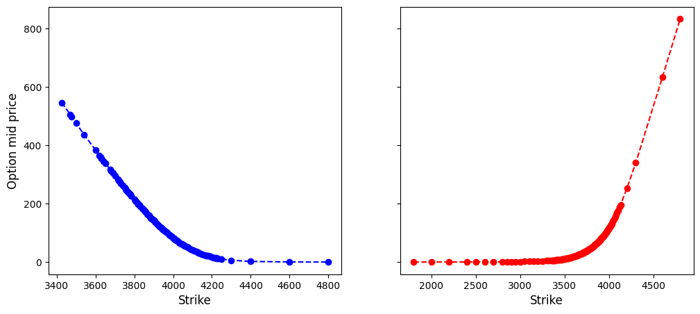

spx_opt.plot_parity()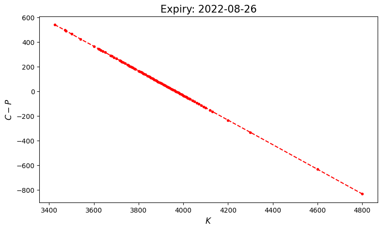

spx_opt.s_adj

3956.9116921934447

spx_opt.imp_vols()

C:\Windows\Temp\ipykernel_3812\903028481.py:94: FutureWarning: Series.__getitem__ treating keys as positions is deprecated. In a future version, integer keys will always be treated as labels (consistent with DataFrame behavior). To access a value by position, use `ser.iloc[pos]`
  s_adj, pv = result.params[0], -result.params[1]

{'imp_vols': array([0.30600045, 0.30595555, 0.2977905 , 0.29545201, 0.28072122,
        0.28232929, 0.2760224 , 0.27571335, 0.26859412, 0.26908309,
        0.27284159, 0.2708769 , 0.26853801, 0.26566743, 0.26527454,
        0.26282943, 0.26242285, 0.2594965 , 0.25959885, 0.25941643,
        0.25750019, 0.25653246, 0.25254566, 0.25387708, 0.25385611,
        0.2507587 , 0.25183417, 0.24960497, 0.24816526, 0.24549749,
        0.2473746 , 0.24511455, 0.24306506, 0.24344569, 0.24239335,
        0.2381772 , 0.23923107, 0.23911993, 0.23822523, 0.23924822,
        0.23345209, 0.23237829, 0.2344444 , 0.23344536, 0.22909791,
        0.22899399, 0.23093383, 0.23010241, 0.22853441, 0.22734051,
        0.22629503, 0.22473931, 0.22267772, 0.22467133, 0.22094489,
        0.22158022, 0.22029972, 0.21894173, 0.22040126, 0.21866736,
        0.21803138, 0.21752707, 0.21522827, 0.21498524, 0.21433691,
        0.21338911, 0.21299896, 0.20983357, 0.21131474, 0.20839273,
        0.20862321, 0.20877018, 0.20719259, 0.20584517, 0.20362794,
        0.20224901, 0.20071144, 0.20063567, 0.19902292, 0.19711411,
        0.19699863, 0.19436676, 0.1925327 , 0.18606077, 0.18129871,
        0.1965902 , 0.22174679]),
 'pv': 0.9978522732469026,
 's_adj': 3956.9116921934447}

spx_opt.plot_imp_vols2(), spx_opt.plot_imp_vols1();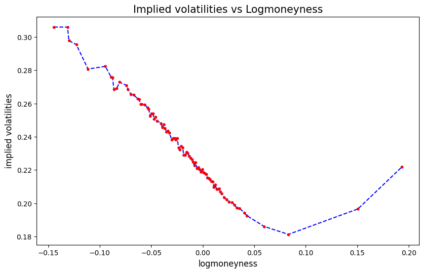

A shorter time to expiry option on SPX

Tips: You may skip this part if you encounter an error.

# choose an expiry 
idx = 5
today = dt.strftime(dt.now(), '%Y-%m-%d')
day_count = (dt.strptime(spx_expiries[idx], '%Y-%m-%d') - dt.now()).days
print(f'option expiry = {spx_expiries[idx]}, today = {today}')
print(f'There are {day_count} days to expiry')
option_chain = spx.option_chain(spx_expiries[idx])
spx_calls1 = option_chain.calls
spx_puts1 = option_chain.puts

option expiry = 2025-08-04, today = 2025-07-28
There are 6 days to expiry

# clean data
spx_calls1 = spx_calls1.dropna()
spx_calls1 = spx_calls1[(spx_calls1['bid'] > 0) & (spx_calls1['ask'] > 0)]
spx_puts1 = spx_puts1.dropna()
spx_puts1 = spx_puts1[(spx_puts1['bid'] > 0) & (spx_puts1['ask'] > 0)]

today = dt.now()
spx_opt1 = OptionAnalytics([spx_calls1, spx_puts1], spx_expiries[idx], today)

C:\Windows\Temp\ipykernel_3812\903028481.py:94: FutureWarning: Series.__getitem__ treating keys as positions is deprecated. In a future version, integer keys will always be treated as labels (consistent with DataFrame behavior). To access a value by position, use `ser.iloc[pos]`
  s_adj, pv = result.params[0], -result.params[1]

spx_opt1.plot_arb()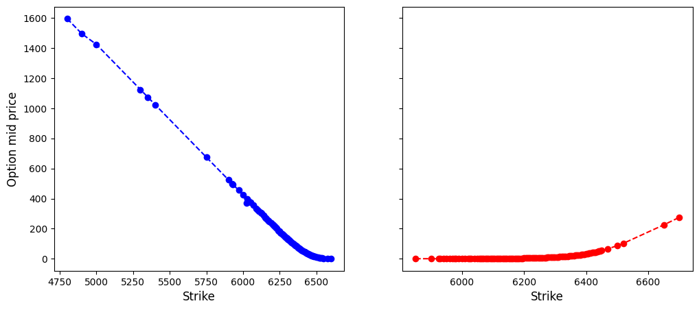

spx_opt1.plot_parity()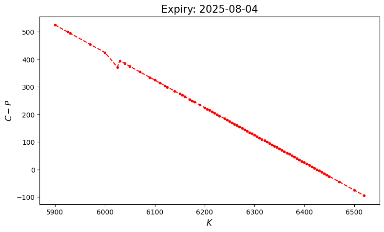

spx_opt.imp_vols()['pv']

C:\Windows\Temp\ipykernel_3812\903028481.py:94: FutureWarning: Series.__getitem__ treating keys as positions is deprecated. In a future version, integer keys will always be treated as labels (consistent with DataFrame behavior). To access a value by position, use `ser.iloc[pos]`
  s_adj, pv = result.params[0], -result.params[1]

0.9978522732469026

spx_opt1.s_adj, spx_opt1.imp_vols()['pv']

C:\Windows\Temp\ipykernel_3812\903028481.py:94: FutureWarning: Series.__getitem__ treating keys as positions is deprecated. In a future version, integer keys will always be treated as labels (consistent with DataFrame behavior). To access a value by position, use `ser.iloc[pos]`
  s_adj, pv = result.params[0], -result.params[1]

(6384.272448907927, 0.9936040369548137)

spx_opt1.plot_imp_vols2(), spx_opt1.plot_imp_vols1();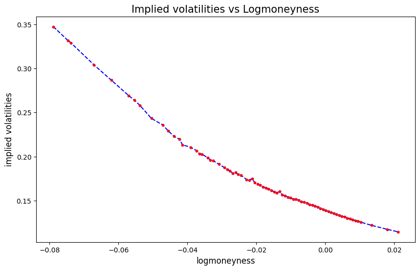

You may start from here.

GPR fit for SPX implied volatility curve

# The posterior mean function from GPR
# inputs: 
# m: prior mean function 
# k: prior kernel
# y: observations
# x: indices
# 
# output: the posterior mean function

def pos_mean(m, k, y, x, sigma=0.001):
    n = len(x)
    
    # calculate the covariance matrices
    tmp, _ = np.meshgrid(x, x)
    Sigma_YY = k(tmp, _)
    Sigma_YY = Sigma_YY + sigma**2*np.identity(n)
    
    # determine Sigma_YY_inv(Y - EY) by solving the linear system Sigma_YY x = Y - EY
    Sigma_YY_inv_Y_EY = np.linalg.solve(Sigma_YY, y - m(x))
    
    # return the posterior mean function
    return lambda xx: m(xx) + sum(k(xx, x)*Sigma_YY_inv_Y_EY)


# The posterior kernel from GPR
# inputs: 
# k: prior kernel
# x: indices
# 
# output: the posterior kernel

def pos_kernel(k, x, sigma=0.1):
    n = len(x)
    
    # calculate the covariance matrices
    tmp, _ = np.meshgrid(x, x)
    Sigma_YY = k(tmp, _)
    Sigma_YY = Sigma_YY + sigma**2*np.identity(n)
    
    # return the posterior kernel
    def _(xx, xp):
        # determine Sigma_YY_inv Sigma_Yxp by solving the linear system Sigma_YY x = Sigma_Yxp
        Sigma_YY_inv_Yxp = np.linalg.solve(Sigma_YY, k(xp, x))
        Sigma_xY = k(xx, x)
        return k(xx, xp) - sum(Sigma_xY*Sigma_YY_inv_Yxp)
        
    return _

imp_vols = spx_opt.ivs
logmnyns = np.log(spx_opt.ks/spx_opt.s_adj)

# set hyperparameters by guessing
A, l, sigma = 0.1, 0.1, 0.01

# prior mean function
# set prior mean as sample mean of implied vols
iv_mean = imp_vols.mean()
mpr = lambda x: iv_mean

# prior kernel
k = lambda x, y: A*np.exp(-np.abs(x-y)**2/2/l**2)

# indices and observations
x_is = logmnyns
n = len(x_is)
y_is = imp_vols

# posterior mean function for implied vol
mpo_iv = pos_mean(mpr, k, y_is, x_is, sigma=sigma)
mpo_iv = np.vectorize(mpo_iv)
mpo_iv(x_is)


# fitted values
iv_hat = mpo_iv(x_is)
pd.DataFrame(y_is, iv_hat)

	0
0.307461	0.306000
0.299448	0.305956
0.298590	0.297790
0.294401	0.295452
0.288030	0.280721
...	...
0.192479	0.192533
0.185995	0.186061
0.181538	0.181299
0.196908	0.196590
0.221521	0.221747

87 rows × 1 columns

# plot 
plt.figure(figsize=(9, 6))
plt.plot(x_is, y_is, 'bo', label='Market data')
plt.xlabel('logmoneyness')
plt.ylabel('implied vol')
x = np.linspace(x_is.min(), x_is.max(), 200)
plt.plot(x, mpo_iv(x), 'r--', label='GPR fit')
plt.legend();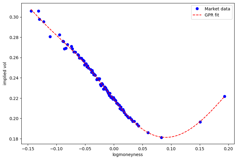

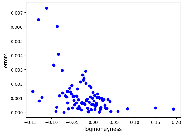
# analysis on absolute errors 
abs_errs = np.abs(iv_hat - y_is)
plt.plot(x_is, abs_errs, 'bo')
plt.xlabel('logmoneyness', fontsize=12) 
plt.ylabel('errors', fontsize=12)
pd.DataFrame(abs_errs).describe().transpose()

	count	mean	std	min	25%	50%	75%	max
0	87.0	0.001156	0.001303	0.000011	0.000347	0.000829	0.001325	0.007309

Fine tune hyperparameters by MLE

# estimate the hyperparameters by MLE

# objective function
def obj(x, y):
    def _(params):
        A, l, sigma = params
        k = lambda u, v: A*np.exp(-np.abs(u-v)**2/2/l**2)
        n = len(x)
        # calculate the covariance matrices
        tmp, _ = np.meshgrid(x, x)
        Sigma_YY = k(tmp, _)
        Sigma_YY = Sigma_YY + sigma**2*np.identity(n)
        Sigma_YY_inv_y = np.linalg.solve(Sigma_YY, y)        
        return np.log(np.linalg.det(Sigma_YY)) + sum(y*Sigma_YY_inv_y) #this is in fact negative log likelihood
    return _

from scipy.optimize import minimize

%%time
# minimize objective function
print(obj(x_is, y_is)([0.1, 0.1, 0.1]))
pars = [0.1, 0.1, 0.1]
res = minimize(obj(x_is, y_is), pars, method='nelder-mead', 
               options={'xatol': 1e-8, 'disp': True}) 
hyparams = res.x
hyparams

-381.2423169273305

C:\Windows\Temp\ipykernel_3812\1457444304.py:14: RuntimeWarning: divide by zero encountered in log
  return np.log(np.linalg.det(Sigma_YY)) + sum(y*Sigma_YY_inv_y) #this is in fact negative log likelihood
d:\HuaweiMoveData\Users\平面向皮卡丘\Desktop\24-25-3\量化金融专题\slides\.venv\Lib\site-packages\scipy\optimize\_optimize.py:869: RuntimeWarning: invalid value encountered in subtract
  np.max(np.abs(fsim[0] - fsim[1:])) <= fatol):

CPU times: total: 18.2 s
Wall time: 9.85 s

<timed exec>:4: RuntimeWarning: Maximum number of function evaluations has been exceeded.

array([ 0.13481481,  0.16574074, -0.00740741])

# hyperparameters estimated from MLE
A, l, sigma = hyparams

# prior mean function
# set prior mean as sample mean of implied vols
iv_mean = imp_vols.mean()
mpr = lambda x: iv_mean

# prior kernel
k = lambda x, y: A*np.exp(-np.abs(x-y)**2/2/l**2)

# indices and observations
x_is = logmnyns
n = len(x_is)
y_is = imp_vols

# posterior mean function for implied vol
mpo_iv = pos_mean(mpr, k, y_is, x_is, sigma=sigma)
mpo_iv = np.vectorize(mpo_iv)
#mpo_iv(x_is)

# plot 
plt.figure(figsize=(9, 6))
plt.plot(x_is, y_is, 'bo', label='Market data')
plt.xlabel('logmoneyness')
plt.ylabel('implied vol')
x = np.linspace(x_is.min(), x_is.max(), 200)
plt.plot(x, mpo_iv(x), 'r--', label='GPR fit')
plt.legend();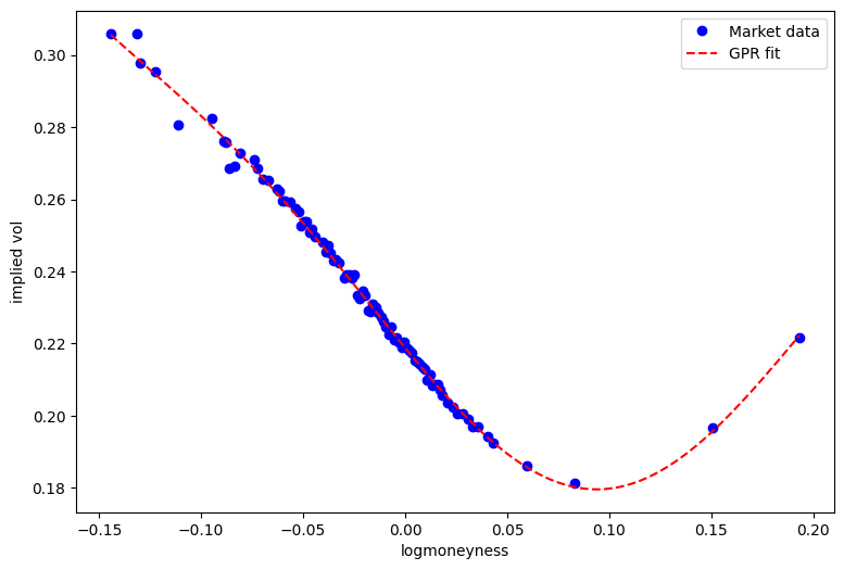

# analysis on absolute errors 
abs_errs = np.abs(iv_hat - y_is)
plt.plot(x_is, abs_errs, 'bo')
plt.xlabel('logmoneyness', fontsize=12) 
plt.ylabel('errors', fontsize=12)
pd.DataFrame(abs_errs).describe().transpose()

	count	mean	std	min	25%	50%	75%	max
0	87.0	0.001156	0.001303	0.000011	0.000347	0.000829	0.001325	0.007309

What is VIX?

Quote from this page in Investopedia:

Created by the Chicago Board Options Exchange (CBOE), the Volatility Index, or VIX, is a real-time market index that represents the market’s expectation of 30-day forward-looking volatility. Derived from the price inputs of the S&P 500 index options, it provides a measure of market risk and investors’ sentiments. It is also known by other names like “Fear Gauge” or “Fear Index.” Investors, research analysts and portfolio managers look to VIX values as a way to measure market risk, fear and stress before they take investment decisions.

Introduced in 1993, the Volatility Index (VIX) was initially a weighted measure of the implied volatility (IV) of eight S&P 100 at-the-money put and call options. Ten years later, in 2004, it expanded to use options based on a broader index, the S&P 500. This expansion allows for a more accurate view of investors’ expectations on future market volatility. VIX values higher than 30 are usually associated with a significant amount of volatility as a result of investor fear or uncertainty. Values below 15 ordinarily correspond to less stressful, or even complacent, times in the markets.

Originally, the VIX computation was designed to mimic the implied volatility of an at-the-money 1 month option on the OEX index. It did this by averaging volatilities from 8 options (puts and calls from the closest to ATM strikes in the nearest and next to nearest months).
The CBOE changed the VIX computation: “CBOE is changing VIX to provide a more precise and robust measure of expected market volatility and to create a viable underlying index for tradable volatility products.”
CBOE listed futures on the VIX in 2004.

Volatility indices published by CBOE

In addition to VIX, other volatility indices published by CBOE include

VIX9D
VIX3M
VIX6M
VOX
VXD: Dow Jones index volatility
RVX
VXN
VVIX: VIX of VIX.

指数	标的资产	期限	用途
VIX9D	标普 500	9 天	短期市场波动对冲
VIX3M	标普 500	3 个月	中长期波动管理
VIX6M	标普 500	6 个月	长期波动对冲
VOX	纳斯达克 100	30 天	科技股波动监测
VXD	道琼斯工业平均指数	30 天	蓝筹股波动监测
RVX	房地产投资信托 (REITs)	30 天	房地产市场波动监测
VXN	纳斯达克综合指数	30 天	科技股及小型股波动监测
VVIX	VIX 指数本身	30 天	波动率的波动性 (市场恐慌指标)

Note

More volatility indices published by CBOE can be found in this link.

VIX Chart from Investopedia

“Formula of financial engineering”

Engineering: “Build something new out of something that is not.”

Notice that all payoffs we saw before can be expressed as a combination of payoffs from calls and puts, even the underlying itself since it can be regarded as a call struck at zero. A natural question to ask is, to what extent, can a given payoff function be represented as a combination of calls and puts?

The answer is surprisingly “all the payoffs”! The following formula shows how.

Let $\varphi$ be a payoff function, we have

\[ \varphi(s) = \varphi(f) + \varphi'(f)(s - f) + \int_f^\infty (s - k)^+ \varphi''(k) \mathrm{d}k + \int_0^f (k - s)^+ \varphi''(k)\mathrm{d}k. \]

Let $\delta$ denote the Dirac delta function and $\theta$ the Heaviside function. Note that heuristically $\theta' = \delta$, i.e., the Dirac delta can be regarded as the derivative of the Heaviside function.

The payoff $\varphi(s)$ at time $T$ can be written as

\[\begin{aligned} \varphi(s) &= \int_0^\infty \varphi(k) \delta(s - k)\,\mathrm{d}k \\ &= \int_0^f \varphi(k) \delta(s - k)\,\mathrm{d}k + \int_f^\infty \varphi(k) \delta(s - k)\,\mathrm{d}k \\ &= \varphi(f) - \int_0^f \varphi'(k) \theta(k - s)\,\mathrm{d}k + \int_f^\infty \varphi'(k) \theta(s - k)\,\mathrm{d}k \\ &= \varphi(f) + \varphi'(f) (s - f) + \int_0^f \varphi''(k) (k - s)^+\,\mathrm{d}k + \int_f^\infty \varphi''(k) (s - k)^+\,\mathrm{d}k. \end{aligned}\]

Thus,

\[ \varphi(S_T) = \varphi(f) + \varphi'(f) (S_T - f) + \int_0^f \varphi''(k) (k - S_T)^+ \mathrm{d}k + \int_f^\infty \varphi''(k) (S_T - k)^+ \mathrm{d}k. \]

With $f = \Eof{S_T}$ and taking expectation on both sides, we end up

\[\begin{aligned} \E[\varphi(S_T)] &= \varphi(f) + \int_0^f \varphi''(k) P(k)\, \mathrm{d}k + \int_f^\infty \varphi''(k) C(k)\, \mathrm{d}k. \end{aligned}\]

The price of any European style contingent claim can be expressed in terms of strips of out-of-money European options.

Remark

Dirac delta function $\delta$ is a distribution, not a function. It is defined by the property that for any continuous function $f$, we have \[ \int_{-\infty}^\infty f(x) \delta(x - a)\,\mathrm{d}x = f(a). \]

Dirac delta function

Heaviside function $\theta$ is defined as $\theta(x) = 0$ for $x < 0$ and $\theta(x) = 1$ for $x \geq 0$. It is the integral of the Dirac delta function, i.e., $\theta'(x) = \delta(x)$.

严格定义: 令 $\delta_1(x), \delta_2(x), ...$ 为一个连续实函数的序列. 若 $\delta_n(x)$ 满足以下两个条件, 那么我们把该函数列称为狄拉克 $\delta$ 函数 (列):

对所有性质良好 (例如在 $x=0$ 连续) 的 $f(x)$ , 都有 \[ \lim_{n \to \infty} \int_{-\infty}^\infty f(x) \delta_n(x)\,\mathrm{d}x = f(0). \]

Example - log contract

Consider the log contract $\displaystyle \varphi(s) = \log s$. Since $\displaystyle \varphi'(s) = \frac1s$ and $\displaystyle \varphi''(s) = -\frac1{s^2}$, we obtain

\[ \log s = \log f + \frac{s - f}{f} - \int_0^f \frac{(k - s)^+}{k^2} \mathrm{d}k - \int_f^\infty \frac{(s - k)^+}{k^2} \mathrm{d}k. \]

Thus,

\[ \Eof{\log S_T} = \log f - \int_0^f \, \frac{P(k)}{k^2} \,\mathrm{d}k - \int_f^\infty\, \frac{C(k)}{k^2} \,\mathrm{d}k. \]

On the other hand, assume $S_t$ satisfies the SDE under risk neutral probability with zero interest and dividend rates

\[ \frac{\mathrm{d}S_t}{S_t} = \sigma_t \mathrm{d}W_t, \]

by applying Ito’s formula to $\log S_t$, we obtain

\[ \log S_T = \log S_0 + \int_0^T \sigma_t \, \mathrm{d}W_t - \frac{1}{2} \int_0^T \sigma_t^2 \, \mathrm{d}t. \]

It follows by taking expectation on both sides that

\[ \Eof{\log S_T} = \log S_0 - \frac12 \Eof{\int_0^T \sigma_t^2 \mathrm{d}t} \]

Compare the two identities we obtain

\[ \frac1T \Eof{\int_0^T \sigma_t^2 \mathrm{d}t} = \frac2T \int_0^f \, \frac{P(k)}{k^2} \,\mathrm{d}k + \frac2T \int_f^\infty\, \frac{C(k)}{k^2} \,\mathrm{d}k. \]

注: 这个式子的左端就是 VIX 的新的定义. “The new VIX squared approximates the conditional risk-neutral expectation of the annualized return variance over the next 30 calendar days.” (Carr and Wu 2004)

Note

Modulo the diffusion process assumption on the underlying, the last relationship is model-free.
VIX is calculated based on this formula with $T$ equal to a month.

注: $\Eof{(s-k)^+} = C(k)$, $\Eof{(k-s)^+} = P(k)$. 这里的 $C(k)$ 代表的是行权价为 $k$ 的 call 期权的价格, 而 $P(k)$ 代表的是行权价为 $k$ 的 put 期权的价格.

Forward price $F$ is defined as the price of a forward contract that delivers one unit of the underlying at time $T$. It is given by \[ F = S e^{-(d-r)\tau} = S e^{-r\tau} e^{-d\tau}. \]

Here, $S$ represents the current price of the underlying, $d$ is the dividend yield, $r$ is the risk-free interest rate, and $\tau$ is the time to maturity in years.

How is VIX calculated?

VIX definition in the CBOE white paper:

\[\text{VIX}^2=\frac{2}{T}\,\sum_i\,\frac{\Delta K_i}{K_i^2}\, Q_i(K_i)\,-\,\frac{1}{T}\,\left[\frac{F}{K_0}-1\right]^2 \]

where $Q_i$ is the price of the out-of-the-money option with strike $K_i$ and $K_0$ is the highest strike below the forward price $F$. $T$ is one month.

注: 在理论上, 积分是从执行价 $k=0$ 一直走到 $+\infty$, 以 $F$ 作为“切点”来拼接看跌和看涨期权部分. 但实际操作中, 缺乏一个连续 $k$ 的期权价格曲线, 必须离散化并使用最近的实际执行价 $K_0$ 来近似 cutting price. 由于 $K_0$ 不一定等于 $F$, 就会产生一项偏差, 这项偏差正是: \[ \frac{1}{T}\,\left(\frac{F}{K_0}-1\right)^2 \]

Simple explanation of VIX formula is that it is a square root of weighted sum of out of the money SPX options.

Quotes by 于鹏

期权价格反应了当前市场的供需状况. 某个到日期的期权价格反应投资者对这段期间内市场波动的预期, 用真金白银报价出来的波动预期. 而与 in-the-money (实值) 期权比起来, 虚值期权没有内在价值, 只有时间价值. 也就是说虚值期权的价格“更纯粹”的反应了这种预期的价值. 那么用虚值期权来计算 VIX, 更契合其设计目的 (VIX is a measure of expected volatility calculated as ..) 还有一个地方也反应了这点, 没有 bid 报价的虚值期权也不会被列入计算之内, “Only SPX options quoted with non-zero bid prices are used in the VIX calculation”. 意味着没有市场需求的期权没有考虑进来的必要.

CBOE’s Volatility Index Mathematics Methodology:

The generalized formula used in the volatility calculation is:

\[ \sigma^2 = \frac{2}{T} \sum_{i} \frac{\Delta K_i}{K_i^2} e^{RT} Q(K_i) - \frac{1}{T} \left( \frac{F}{K_0} - 1 \right)^2 \]

where:

$\sigma$: Volatility index = $\sigma \times 100$
$T$: Time to expiration (in years), Number of minutes from time of calculation until expiration / Number of minutes in a 365-day year (365 x 1,440 = 525,600).
$F$: Option-implied forward price. It can be calculated by the intercept of Call-Put Parity’s OLS regression. Or it can be calculated by identifying the options strike price at which the absolute difference between the call price and the put price is smallest. And thus $F = \text{Stike Price} + e^{RT} (\text{Call Price} - \text{Put Price})$.
$R$: Risk-free interest rate to expiration.
$K_0$: First strike equal to or otherwise immediately below $F$.
$K_i$: Strike price of the $i$-th out-of-the-money option.
- A call if $K_i > K_0$;
- A put if $K_i < K_0$;
- both calls and puts if $K_i = K_0$.
$\Delta K_i$: Interval between strike spreads.
- Highest OTM Strike $K_i$: $K_i - K_{i-1}$;
- Lowest OTM Strike $K_i$: $K_{i+1} - K_i$;
- Otherwise: $(K_{i+1} - K_{i-1})/2$.
$Q(K_i)$: Option price of the OTM option with strike $K_i$. $Q(K_0)$ is the average of the call and put prices at strike $K_0$.

Download VIX data from `yfinance`

You may skip this part if you encounter an error.

start = '2007-01-01'
end = '2022-07-29'
vix = yf.download('^VIX', start=start, end=end)
vix = vix.drop('Volume', axis=1)
vix

C:\Windows\Temp\ipykernel_3812\3558120957.py:3: FutureWarning: YF.download() has changed argument auto_adjust default to True
  vix = yf.download('^VIX', start=start, end=end)
[*********************100%***********************]  1 of 1 completed

Price	Close	High	Low	Open
Ticker	^VIX	^VIX	^VIX	^VIX
Date
2007-01-03	12.040000	12.750000	11.530000	12.160000
2007-01-04	11.510000	12.420000	11.280000	12.400000
2007-01-05	12.140000	12.250000	11.680000	11.840000
2007-01-08	12.000000	12.830000	11.780000	12.480000
2007-01-09	11.910000	12.470000	11.690000	11.860000
...	...	...	...	...
2022-07-22	23.030001	23.809999	22.410000	23.299999
2022-07-25	23.360001	24.570000	23.190001	24.330000
2022-07-26	24.690001	25.309999	23.820000	23.950001
2022-07-27	23.240000	24.410000	23.020000	24.270000
2022-07-28	22.330000	23.540001	22.219999	23.330000

3920 rows × 4 columns

plt.figure(figsize=(9, 6))
vix['Close'].plot(label='VIX')
#plt.plot(spx_vol*100, 'r-.', label='Historical Volatility')
plt.grid()
plt.legend();

<Figure size 900x600 with 0 Axes>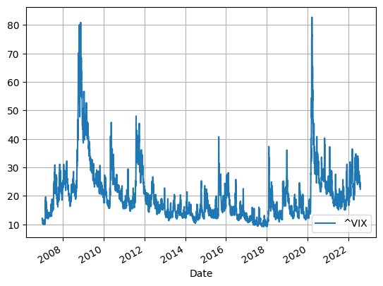

# plot log(vix)
plt.figure(figsize=(9, 6))
log(vix)['Close'].plot(label='log ViX')
plt.grid()
plt.legend();

<Figure size 900x600 with 0 Axes>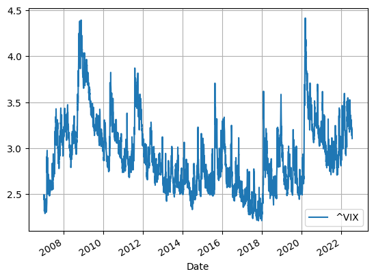

Volatility derivatives

variance swap
volatility swap
VIX futures
VIX options

Variance swap

Quote from the Wikipage:

A variance swap is an over-the-counter financial derivative that allows one to speculate on or hedge risks associated with the magnitude of movement, i.e. volatility, of some underlying product, like an exchange rate , interest rate, or stock index.

One leg of the swap will pay an amount based upon the realized variance of the price changes of the underlying product. Conventionally, these price changes will be daily log returns, based upon the most commonly used closing price. The other leg of the swap will pay a fixed amount, which is the strike, quoted at the deal’s inception. Thus the net payoff to the counterparties will be the difference between these two and will be settled in cash at the expiration of the deal, though some cash payments will likely be made along the way by one or the other counterparty to maintain agreed upon margin.

In summary, a variance swap is a forward contract on realized (annualized) variance whose payoff function ideally is given by

\[ N \times \left(\frac1T \int_0^T \sigma_t^2 \mathrm{d}t - K \right) \]

where $K$ is the strike and $N$ denotes the notional.

Volatility swap

Quote from the Wikipage:

In finance, a volatility swap is a forward contract on the future realised volatility of a given underlying asset. Volatility swaps allow investors to trade the volatility of an asset directly, much as they would trade a price index.

The underlying is usually a foreign exchange (FX) rate (very liquid market) but could be as well a single name equity or index. However, the variance swap is preferred in the equity market because it can be replicated with a linear combination of options and a dynamic position in futures.

Unlike a stock option, whose volatility exposure is contaminated by its stock price dependence, these swaps provide pure exposure to volatility alone. This is truly the case only for forward starting volatility swaps. However, once the swap has its asset fixings its mark-to-market value also depends on the current asset price. One can use these instruments to speculate on future volatility levels, to trade the spread between realized and implied volatility, or to hedge the volatility exposure of other positions or businesses.

In summary, a volatility swap is a forward contract on realized (annualized) volatility whose payoff function ideally is given by

\[ N \times \left(\sqrt{\frac1T \int_0^T \sigma_t^2 \mathrm{d}t} - K \right) \]

where $K$ is the strike and $N$ denotes the notional.

Calculating volatility swap fair strike from MGF

By applying the following formula

\[ \sqrt x = \frac1{2\sqrt\pi}\int_0^\infty s^{-\frac32}\left(1 - e^{-xs}\right) \mathrm{d}s, \]

we obtain

\[ \Eof{\sqrt{\frac1T \int_0^T \sigma_t^2 \mathrm{d}t}} = \frac1{2\sqrt\pi}\int_0^\infty s^{-\frac32}\left(1 - \Eof{e^{-xs}}\right) \mathrm{d}s \]

where apparently,

\[ x = \frac1T \int_0^T \sigma_t^2 \mathrm{d}t \]

and $\Eof{e^{-xs}}$ the moment generating function for realized variance.

VIX futures

According to the VIX page on CBOE,

Introduced in 2004 on Cboe Futures Exchange (CFE), VIX futures provide market participants with the ability to trade a liquid volatility product based on the VIX Index methodology. VIX futures reflect the market’s estimate of the value of the VIX Index on various expiration dates in the future. VIX futures provide market participants with a variety of opportunities to implement their view using volatility trading strategies, including risk management, alpha generation and portfolio diversification.

VIX option

Quote from this page in Invstopeida

A VIX option is a non-equity index option that uses the CBOE Volatility Index as its underlying asset. Call and put VIX options are both available. The call options hedge portfolios against a sudden market decline, and put options hedge against a rapid reversal of short positions on the S&P 500 index. These options thus allow traders and investors to speculate on future moves in volatility.

A look at the VIX option chain from Yahoo Finance

Visit this Yahoo Finance link for VIX option chain.

You may skip the next 5 cells if you encounter an error.

vix = yf.Ticker('^VIX')
vix_expiries = vix.options
print(vix_expiries)

('2025-07-30', '2025-08-06', '2025-08-13', '2025-08-20', '2025-08-27', '2025-09-17', '2025-10-22', '2025-11-19', '2025-12-17', '2026-01-21', '2026-02-18', '2026-03-18', '2026-04-15')

# choose an expiry 
idx = 4
today = dt.strftime(dt.now(), '%Y-%m-%d')
day_count = (dt.strptime(vix_expiries[idx], '%Y-%m-%d') - dt.now()).days
print(f'option expiry = {vix_expiries[idx]}, today = {today}')
print(f'There are {day_count} days to expiry')
option_chain = vix.option_chain(vix_expiries[idx])
vix_calls, vix_puts = option_chain.calls, option_chain.puts

option expiry = 2025-08-27, today = 2025-07-28
There are 29 days to expiry

# clean data
vix_calls = vix_calls.drop(['currency', 'contractSize'], axis = 1).dropna()
vix_calls = vix_calls[(vix_calls['bid'] > 0) & (vix_calls['ask'] > 0)]
vix_calls

	contractSymbol	lastTradeDate	strike	lastPrice	bid	ask	change	percentChange	volume	openInterest	impliedVolatility	inTheMoney
5	VIXW250827C00018000	2025-07-25 19:54:01+00:00	18.0	2.0	0.9	2.35	0.0	0.0	103.0	0	1.535159	False
6	VIXW250827C00019000	2025-07-25 20:11:19+00:00	19.0	1.7	0.7	2.03	0.0	0.0	88.0	0	1.523440	False

vix_puts = vix_puts.drop(['currency', 'contractSize'], axis = 1).dropna()
vix_puts = vix_puts[(vix_puts['bid'] > 0) & (vix_puts['ask'] > 0)]
vix_puts

	contractSymbol	lastTradeDate	strike	lastPrice	bid	ask	change	percentChange	volume	openInterest	impliedVolatility	inTheMoney
7	VIXW250827P00020000	2025-07-25 13:46:04+00:00	20.0	2.63	2.13	3.9	0.0	0.0	1.0	0	0.00001	True

# save data
#vix_calls.to_csv('vixcall_07252022.csv', index=False)
#vix_puts.to_csv('vixput_07252022.csv', index=False)

You may start from here.

# read in saved data
vix_calls = pd.read_csv('vixcall_07252022.csv')
vix_puts = pd.read_csv('vixput_07252022.csv')

expiry, today = '2022-08-24', '2022-07-25'
vix_opt = OptionAnalytics([vix_calls, vix_puts], expiry, today)
#vix_opt = OptionAnalytics([vix_calls, vix_puts], vix_expiries[idx], dt.now())

C:\Windows\Temp\ipykernel_3812\903028481.py:94: FutureWarning: Series.__getitem__ treating keys as positions is deprecated. In a future version, integer keys will always be treated as labels (consistent with DataFrame behavior). To access a value by position, use `ser.iloc[pos]`
  s_adj, pv = result.params[0], -result.params[1]

vix_opt.plot_arb()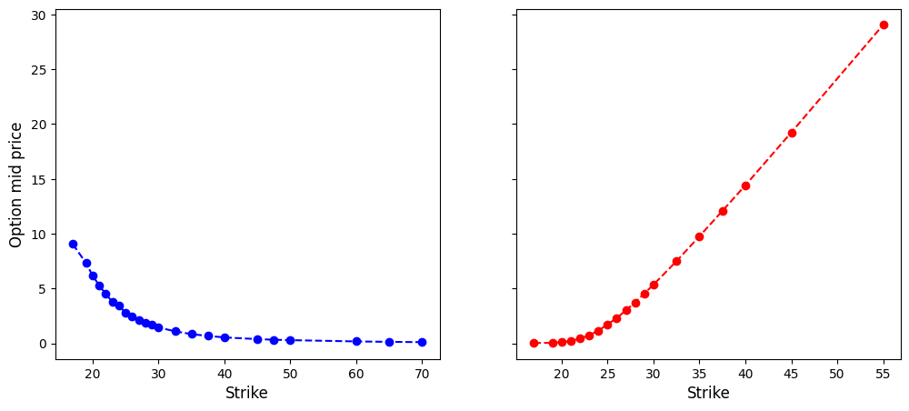

vix_opt.plot_parity()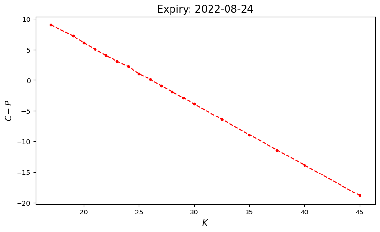

vix_opt.plot_imp_vols2(), vix_opt.plot_imp_vols1();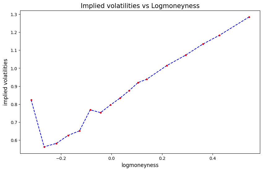

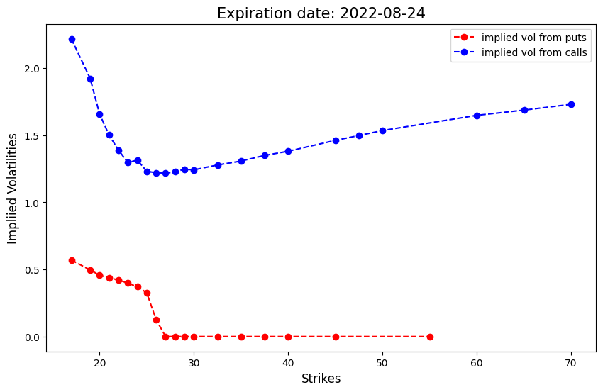
GPR fit for VIX option implied volatility curve

imp_vols = vix_opt.ivs[1:]
#imp_vols = vix_opt.ivs
logmnyns = np.log(vix_opt.ks[1:]/vix_opt.s_adj)

# set hyperparameters by guessing
sigma, A, l = 0.05, 0.1, 0.1

# prior mean function
# set prior mean as sample mean of implied vols
iv_mean = imp_vols.mean()
mpr = lambda x: iv_mean

# prior kernel
k = lambda x, y: A*np.exp(-np.abs(x-y)**2/2/l**2)

# indices and observations
x_is = logmnyns
n = len(x_is)
y_is = imp_vols

# posterior mean function for implied vol
mpo_iv = pos_mean(mpr, k, y_is, x_is, sigma=sigma)
mpo_iv = np.vectorize(mpo_iv)
mpo_iv(x_is)


# fitted values
iv_hat = mpo_iv(x_is)
pd.DataFrame(y_is, iv_hat)

	0
0.794121	0.823381
0.612930	0.562470
0.561423	0.581719
0.612908	0.626235
0.685567	0.651083
0.736006	0.768180
0.767337	0.752712
0.796917	0.795185
0.833553	0.833420
0.874426	0.875310
0.912757	0.919806
0.945017	0.938292
1.010601	1.014723
1.074513	1.072477
1.127997	1.134668
1.184969	1.182831
1.275277	1.285238

# plot 
plt.figure(figsize=(9, 6))
plt.plot(x_is, y_is, 'bo', label='Market data')
plt.xlabel('logmoneyness')
plt.ylabel('implied vol')
x = np.linspace(x_is.min(), x_is.max(), 200)
plt.plot(x, mpo_iv(x), 'r--', label='GPR fit')
plt.legend();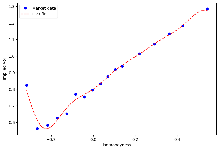

# analysis on absolute errors 
abs_errs = np.abs(iv_hat - y_is)
plt.plot(x_is, abs_errs, 'bo')
plt.xlabel('logmoneyness', fontsize=12) 
plt.ylabel('errors', fontsize=12)
pd.DataFrame(abs_errs).describe().transpose()

	count	mean	std	min	25%	50%	75%	max
0	17.0	0.013887	0.01462	0.000133	0.002138	0.007049	0.020297	0.05046

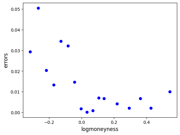
Appendix (Optional)

Volatility estimation using high frequency data

Market microstructure noise may contaminate the data in high frequency, resulting in inconsistency of estimators.

Realized variance

The following estimator is called the Realized Variance (RV) estimator

\[ \sum_{i=1}^n \, \left(Y_{t_i} - Y_{t_{i-1}} \right)^2 = \sum_{i=1}^n \, \left( \Delta Y_{t_i} \right)^2, \]

where $Y_t = \log S_t$ and $S_t$ is the price series of the asset under consideration.

Technical notes

Realized variance and realized covariance
Given a partition $\Pi = \{0 = t_1 < \cdots < t_n=T\}$ of the interval $[0, T]$, the realized variance $[X]_T^\Pi$ of the process $X_t$ sampled at $\Pi$ is defined by \[ [X]_T^\Pi = \sum_{i=1}^n |X_{t_i} - X_{t_{i-1}}|^2. \]

Similiarly, the realized covariance between $X_t$ and $Y_t$ sampled at $\Pi$ is given by

\[ [X, Y]_T^\Pi = \sum_{i=1}^n (X_{t_i} - X_{t_{i-1}})(Y_{t_i} - Y_{t_{i-1}}) \]

Quadratic variation (integrated variance) and covariation
The quadratic variation of $X$ is defined by the limit \[ \angl{X}_t = \lim_{\|\Pi_n\| \to 0} [X]_T^{\Pi_n} \] provided the limit exists. $\Pi_n$ denotes a sequence of partitions of the interval $[0, T]$ such that $\|\Pi_n\| \to 0$ as $n \to \infty$, where $\|\Pi_n\|$ denotes the mesh of the partition $\Pi_n$.

Likewise, the covariation between and $X$ and $Y$ is defined by the limit \[ \angl{X, Y}_t = \lim_{\|\Pi_n\| \to 0} [X, Y]_T^{\Pi_n}. \]

Assumption

The log price $X_t$ follows the Ito process

\[ \mathrm{d}X_t = \mu_t \mathrm{d}t + \sigma_t \mathrm{d}W_t, \] nd where $W_t$ is a Brownian motion. Uer the assumption, $\angl{X}_t = \int_0^t \sigma_\tau^2 \mathrm{d}\tau$.

Integrated variance or quadratic variation

Given a set of tick data, how can we measure the, say daily, variance?
A possibility is to estimate the integrated variance, also known as the quadratic variation in the theory of semimartingale. We shall use both terms interchangeably hereafter.

Recall that the quadratic variation $\angl{X}_t$ of the continuous stochastic process $X_t$ is defined by

\[ \angl{X}_T:= \lim_{\|\Pi_n\| \to 0} \sum_{{t_i} \in \Pi_n} |\Delta X_{t_i}|^2 \]

provided the limit exist (in probability).

Thus, the goal is to estimate the quadratic variation of the efficient log price from the transacted log price, i.e., tick data. However, the subtlety is that efficient is not directly observable and is contaminated by market microstructure noises.

Note

If the process $X$ has jumps, the quadratic variation $\angl{X}$ becomes price
\[\begin{aligned} \langle X \rangle_t &= \langle X^c \rangle_t + \sum_{0 < s \leq t} |\Delta X_s|^2, \end{aligned}\]
where $X^c$ denotes the continuous part of $X$ and $\Delta X_s := X_s - X_{s^-}$ is the jump size at time $s$. In this case, the integrated variance usually refers to $\langle X^c \rangle$, i.e., the quadratic variation of the continuous part.
We shall always assume $X$ is a continuous process, thus no jumps, in the sequel.

Microstructure noise

In the limit of very high sampling frequency, RV picks up mainly the market microstructure noise. To see this, suppose that the observed price $Y_t$ is given by

\[Y_t =X_t +\epsilon_t,\]

where $X_t$ is the value of the underlying (log-)price process of interest and $\epsilon_t$ is a random market microstructure-related noise term, assumed independent of $X_t$. Suppose we sample the price series $n+1$ times (so that there are $n$ price changes) at $\Pi=\{0=t_0 < \cdots < t_n = T\}$ in the time interval $[0, T]$.

Note that, conditioned on $\cF_T^X$, the conditional expectation of the realized variance of transacted (log) price satisties

\[\begin{aligned} \E\left([Y]_T^\Pi \mid \mathcal{F}_T^X\right) &:= \sum_{i=1}^n \E\left((\Delta Y_{t_i})^2 \mid \mathcal{F}_T^X\right) \\ &= \sum_{i=1}^n (\Delta X_{t_i})^2 + 2 \sum_{i=1}^n \Delta X_{t_i} \E\left(\Delta \epsilon_{t_i} \mid \mathcal{F}_T^X\right) + \sum_{i=1}^n \E\left((\Delta \epsilon_{t_i})^2 \mid \mathcal{F}_T^X\right) \\ &= [X]_T + 2 n \, \text{var}[\epsilon] \\ &\approx \langle X \rangle_T + 2 n \, \text{var}[\epsilon]. \end{aligned}\]

Note

The difference between $[X]_T$ and $\angl{X}_T$ is referred to as the discretization error, which is usually controled by the integrated quarticity $\int_0^T \sigma_t^4 \mathrm{d}t$.

Asymptotic result

A more detailed, but more technical, asymptotic analysis shown in [Zhang, Mykland and Aït-Sahalia]^[9] yields that as $n \to \infty$

\[ [Y]^{\Pi}_T \mathop{\approx}^{\mathcal L} \angl{X}_T + 2 \, n \, \text{var}[\epsilon] + \sqrt{ 4 n \Eof{\epsilon^4} + \frac{2T}{n} \int_0^T \sigma_t^4 \mathrm{d}t} \; Z, \]

where $Z \sim N(0,1)$.

Note

The naive RV estimator $[Y]_T^\Pi$ is biased by the variance of market microstructure noise $\epsilon$. The biasedness increases as the sampling frequency $n$ increases.
We see that as $n\to\infty$, the naive RV estimator $[Y]_T^\Pi$ picks up mainly the microstructure noise.

The conventional solution

The conventional solution is to sample at most every five minutes or so.
- For high frequency data, sampling only every 5 minutes usually corresponds to throwing out more than 99% of the points!
To quote [Zhang, Mykland and Aït-Sahalia]^[9], “It is difficult to accept that throwing away data, especially in such quantities, can be an optimal solution.”
From a more practical perspective, if we believe that volatility is time-varying, it makes sense to try and measure it from recent data over the last few minutes rather than from a whole day of trading.

Subsampling

Let $\Pi^{(k)} = \{0 \leq t_0^{(k)} < \cdots < t_{n_k}^{(k)}\leq T\}$, for $1 \leq k \leq K$, be a collection of nonoverlapping subsampling times in $\Pi$. That is,

\[ \bigcup_{k=1}^K \Pi^{(k)} = \Pi \quad \text{ and } \quad \Pi^{(k)} \cap \Pi^{(\ell)} = \emptyset \; \text{for } k \neq \ell. \]

A typical example that we shall be using in the following is by sampling every $K$ ticks from the $k$th tick on. That is,

\[\begin{aligned} \Pi^{(1)} &= \{t_1 < t_{1+K} < t_{1 + 2K} < \cdots < t_{1 + n_1 K} \leq T \}, \\ \Pi^{(2)} &= \{t_2 < t_{2+K} < t_{2 + 2K}< \cdots < t_{2 + n_2 K} \leq T \}, \\ &\quad \vdots \\ \Pi^{(K)} &= \{t_0 < t_K < t_{2K} < \cdots < t_{n_K K} \leq T \}. \end{aligned}\]

We denote by $[Y]_T^{\Pi^{(k)}}$ the RV estimate of $Y$ using the subsamples that are sampled from the sampling times in $\Pi^{(k)}$, for $1 \leq k \leq K$.

By the same token, we have the following asymptotics for each subsample $k \in \{1, \cdots, K\}$

\[ [Y]^{\Pi^{(k)}}_T \mathop{\approx}^{\mathcal L} \angl{X}_T + 2 \, n_k \, \text{var}[\epsilon] + \sqrt{ 4 n_k \Eof{\epsilon^4} + \frac{2T}{n_k} \int_0^T \sigma_t^4 \mathrm{d}t} \; Z_k \]

where $Z_k \sim N(0,1)$.

Boosting RV estimator

We can boost the RV estimator by averaging over the “weak learners” $[Y]_T^{\Pi^{(k)}}$

\[\begin{aligned} [Y]_T^{\text{avg}} &= \frac{1}{K} \sum_{k=1}^K [Y]_T^{\Pi^{(k)}} \\ &\approx \langle X \rangle_T + 2 \, \bar{n}_K \, \text{var}[\epsilon] + \sqrt{ 4 \frac{\bar{n}_K}{K} \E[\epsilon^4] + \frac{4T}{3 \bar{n}_K} \int_0^T \sigma_t^4 \, \mathrm{d}t} \, Z. \end{aligned}\]

where $n_K := 1K _k n_k $ is the average number of ticks in each subsample, roughly equal to $\frac nK$.

Note

Boosting reduces biasedness and variance by a factor of $K$, but is unable to completely remove the biasedness.
The optimal average subsample size $\bar n^*$ is given by \[ \bar n^* = \sqrt[3]{\frac T{6\text{var}^2[\epsilon]} \int_0^T \sigma_t^4 \mathrm{d}t}. \]

Thus, the whole sample set is splitted into roughly $K^* \approx \frac n{\bar n^*}$ sets of subsamples.

The ZMA estimator

Recall that

\[\begin{aligned} [Y]_T^\Pi &\approx \langle X \rangle_T + n \, \text{var}[\epsilon], \\ [Y]_T^{\text{avg}} &\approx \langle X \rangle_T + \bar{n}_K \, \text{var}[\epsilon]. \end{aligned}\]

We can eliminate bias by forming

\[\begin{aligned} \frac{1}{\bar{n}_K}[Y]_T^{\text{avg}} - \frac{1}{n} [Y]_T^\Pi &\approx \left( \frac{1}{\bar{n}_K} - \frac{1}{n} \right) \langle X \rangle_T. \end{aligned}\]

Thus we obtain the [Zhang, Mykland and Aït-Sahalia]^[9] (ZMA) bias-corrected estimator of $\angl{X}_T$:

\[ [Y]_T^{ZMA} := \frac{1}{n - \bar n_K} \, \left\{n \, [Y]_T^{avg} - \bar n_K \, [Y]^\Pi_T \right\}. \]

Moreover, we have the asymptotic behavior for $[Y]_T^{ZMA}$ as

\[ [Y]_T^{ZMA} \approx \angl{X}_T + \frac1{\sqrt[6]n}\sqrt{\frac8{c^2}\text{var}^2[\epsilon] + c \frac{4T}3 \int_0^T \sigma_t^4 \mathrm{d}t} \; Z \]

where $Z \sim N(0,1)$. The optimal constant $c^*$ is given by

\[ c^* = \left(\frac T{12 \, \text{var}^2[\epsilon]} \int_0^T \sigma_t^4 \mathrm{d}t \right)^{-\frac13}. \]

Note

In the original paper [Zhang, Mykland and Aït-Sahalia]^[9], the authors suggested the estimator as $[Y]_T^{avg} - \frac{\bar n_K}{n}[Y]_T^\Pi$, whereas the estimator $[Y]_T^{ZMA}$ obtained above is referred to as the small-sample adjustment in the paper.

The Zhou estimator

Define

\[\begin{align} [Y]_T^{\Pi, Z} &: = \sum_{i=1}^n (\Delta Y_{t_i})^2 + \sum_{i=2}^n \Delta Y_{t_i} \Delta Y_{t_{i-1}} + \sum_{i=1}^{n-1} \Delta Y_{t_i} \Delta Y_{t_{i+1}} \\ &= \sum_{i=1}^n (Y_{t_i} - Y_{t_{i-1}})(Y_{t_{i+1}} - Y_{t_{i-2}}). \end{align}\]

Thus, under the assumption $Y = X + \epsilon$ of serially uncorrelated noise independent of returns $X$, we obtain $\mathbb{E}\left[[Y]^{\Pi, Z}\right] = \Eof{[X]_T}$.

By further assume $X_t = \sigma W_{\tau(t)}$ (a time-changed Brownian motion) for some Brownian motion $W$ and deterministic increasing function $\tau(\cdot)$, since

\[ \Eof{(\Delta X_{t_i})^2} = \sigma^2 \Eof{\left\{ W_{\tau(t_i)} - W_{\tau(t_{i-1})} \right\}^2} = \sigma^2 \{\tau(t_i) - \tau(t_{i-1})\}, \]

we have

\[ \mathbb{E}\left[[Y]^{\Pi, Z}\right] = \sigma^2 \{\tau(T) - \tau(0) \} = \angl{X}_T. \]

In other words, in this case $[Y]^{\Pi, Z}$ is an unbiased estimator of $\angl{X}_T$.

Realized library

Realized Library at Oxford-Man Institute of Quantitative Finance publishes daily realized variances/volatilities for various indices.

https://realized.oxford-man.ox.ac.uk/

Note

Unfortunately, the Realized Library has ceased providing the service.

SPX realized variance

from datetime import datetime as dt

df = pd.read_csv('OxfordManRealizedVolatilityIndices.csv', index_col=0, header=2)
rv1 = pd.DataFrame(index=df.index)
for col in df.columns:
    if col[-3:] == '.rk':
        rv1[col] = df[col]

# convert index into datetime
rv1.index = [dt.strptime(str(date), "%Y%m%d") for date in rv1.index.values]

df

	SPX2.rv	SPX2.rk	SPX2.r	SPX2.rv5ss	SPX2.rv10	SPX2.rv10ss	SPX2.bv5	SPX2.bv5ss	SPX2.medrv	SPX2.rs	...	FTSEMIB.rs	FTSEMIB.rs5ss	FTSEMIB.nobs	FTSEMIB.timespan	FTSEMIB.rcto	FTSEMIB.open	FTSEMIB.highlow	FTSEMIB.highopen	FTSEMIB.openprice	FTSEMIB.closeprice
DateID
20000103	0.000157	0.000161	-0.010104	0.000144	0.000175	0.000170	0.000157	0.000142	0.000084	0.000099	...	0.000323	0.000314	496.0	29752.752	NaN	34152.212	0.061739	0.002525	43900.00	41477.00
20000104	0.000298	0.000264	-0.039292	0.000219	0.000400	0.000247	0.000206	0.000206	0.000092	0.000254	...	0.000144	0.000173	471.0	28319.096	NaN	35524.926	0.020667	0.001046	41072.00	40468.00
20000105	0.000307	0.000305	0.001749	0.000298	0.000258	0.000307	0.000292	0.000279	0.000111	0.000138	...	0.000144	0.000153	497.0	29751.621	NaN	34154.433	-0.029584	0.029584	39000.00	39449.00
20000106	0.000136	0.000149	0.001062	0.000136	0.000108	0.000133	0.000127	0.000127	0.000086	0.000062	...	0.000196	0.000216	496.0	29691.265	NaN	34154.335	0.032678	0.000276	39834.00	38736.00
20000107	0.000093	0.000123	0.026022	0.000112	0.000121	0.000114	0.000083	0.000095	0.000049	0.000024	...	0.000072	0.000081	497.0	29751.482	NaN	34153.093	-0.027410	0.026694	39144.00	40199.00
...	...	...	...	...	...	...	...	...	...	...	...	...	...	...	...	...	...	...	...	...	...
20171129	0.000016	0.000017	-0.000693	0.000017	0.000016	0.000016	0.000012	0.000013	0.000019	0.000009	...	0.000030	0.000025	19553.0	27358.791	NaN	32401.219	0.010438	0.005222	22391.37	22325.94
20171130	0.000028	0.000020	0.004886	0.000023	0.000035	0.000025	0.000024	0.000024	0.000018	0.000010	...	0.000021	0.000024	23672.0	27357.591	NaN	32402.862	0.008467	0.004035	22467.64	22368.29
20171201	0.000088	0.000130	-0.001256	0.000117	0.000120	0.000124	0.000093	0.000126	0.000138	0.000061	...	0.000047	0.000054	25521.0	27359.230	NaN	32400.969	-0.013862	0.008983	22168.37	22106.10
20171204	0.000023	0.000023	-0.006854	0.000021	0.000022	0.000020	0.000024	0.000022	0.000020	0.000014	...	0.000015	0.000015	21585.0	27359.204	NaN	32400.856	0.006576	0.003166	22350.63	22362.11
20171205	NaN	NaN	NaN	NaN	NaN	NaN	NaN	NaN	NaN	NaN	...	NaN	NaN	NaN	NaN	NaN	NaN	NaN	NaN	NaN	NaN

4683 rows × 399 columns

rv1

	SPX2.rk	FTSE2.rk	N2252.rk	GDAXI2.rk	RUT2.rk	AORD2.rk	DJI2.rk	IXIC2.rk	FCHI2.rk	HSI2.rk	...	AEX.rk	SSMI.rk	IBEX2.rk	NSEI.rk	MXX.rk	BVSP.rk	GSPTSE.rk	STOXX50E.rk	FTSTI.rk	FTSEMIB.rk
2000-01-03	0.000161	NaN	NaN	0.000702	0.000264	NaN	0.000135	0.000574	0.000262	0.000261	...	0.000124	NaN	0.000168	NaN	0.000088	0.000404	NaN	0.000272	0.000158	0.000520
2000-01-04	0.000264	0.000249	0.000162	0.000591	0.000232	0.000045	0.000159	0.000575	0.000372	0.000207	...	0.000233	0.000102	0.000215	NaN	0.000214	0.000617	NaN	0.000252	0.000123	0.000336
2000-01-05	0.000305	0.000198	0.000245	0.001081	0.000145	0.000256	0.000196	0.000941	0.000334	0.001597	...	0.000448	0.000123	0.000292	NaN	0.000173	0.000982	NaN	0.000506	0.000394	0.000422
2000-01-06	0.000149	0.000148	0.000198	0.000306	0.000056	0.000031	0.000124	0.000580	0.000248	0.000870	...	0.000224	0.000087	NaN	0.000030	0.000056	0.000501	NaN	0.000110	0.000586	0.000339
2000-01-07	0.000123	0.000126	0.000157	0.000301	0.000031	0.000043	0.000096	0.000396	0.000257	0.000508	...	0.000107	0.000066	0.000155	0.000039	0.000082	0.000258	NaN	0.000149	0.000159	0.000160
...	...	...	...	...	...	...	...	...	...	...	...	...	...	...	...	...	...	...	...	...	...
2017-11-29	0.000017	0.000018	0.000025	0.000047	0.000037	0.000016	0.000012	0.000066	0.000030	0.000039	...	0.000034	0.000021	0.000056	0.000009	0.000035	0.000123	0.000019	0.000040	NaN	0.000029
2017-11-30	0.000020	0.000020	0.000038	0.000058	0.000035	0.000031	0.000026	0.000039	0.000040	0.000040	...	0.000036	0.000033	0.000066	0.000025	0.000042	0.000114	0.000016	0.000044	NaN	0.000033
2017-12-01	0.000130	0.000041	0.000066	0.000142	0.000208	0.000017	0.000153	0.000126	0.000110	0.000066	...	0.000092	0.000056	0.000090	0.000026	0.000061	0.000151	0.000034	0.000117	NaN	0.000073
2017-12-04	0.000023	0.000027	0.000039	0.000050	0.000104	0.000009	0.000024	0.000060	0.000028	0.000082	...	0.000028	0.000026	0.000048	0.000031	0.000050	0.000092	0.000012	0.000064	NaN	0.000029
2017-12-05	NaN	0.000019	0.000027	0.000059	0.000025	0.000018	0.000023	0.000046	0.000037	0.000044	...	0.000026	0.000028	0.000043	0.000026	0.000045	0.000139	0.000009	0.000039	NaN	NaN

4683 rows × 21 columns

# plot spx realized variance
# spx2.rk contains the rv calcuated by the realized kernel within 5-min bins
spx_rv = pd.DataFrame(rv1['SPX2.rk'])
spx_rv.plot(color='red', grid=True, title='SPX realized variance',
         figsize=(12, 6), ylim=(0,0.003));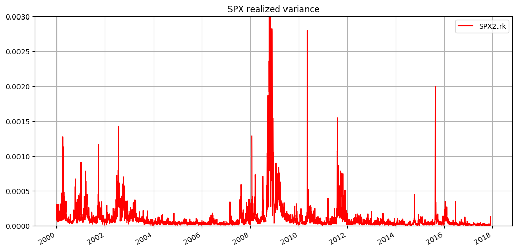

The Corsi HAR-RV forecast

The Corsi HAR-RV model implements a regression to fit the parameters.
This model can be regarded as a poor man’s version of a long memory model such as ARFIMA.
- True long-memory models such as ARFIMA are notoriously hard to fit.
HAR-RV can also be considered an intelligent alternative to GARCH.
The model boils down to the regression

\[RV_{t,t+h} = \beta_0 + \beta_D\,RV_t + \beta_W\,RV_{t-5,t} + \beta_M\,RV_{t-22,t} + \epsilon_{t,t+h}.\]

In words, the RV forecast for $h$ days from now is a linear combination of the current realized variance and (aggregate) RV estimates for the last week and the last month.

Note

$RV$ denotes the logarithm of realized variance.

import statsmodels.formula.api as sm

# take h = 1 in the HAR-RV model
# y = RV_{t+h}
# rv1 = RV_t
# rv5 = RV_{t-5}
# rv22 = RV_{t-22}
spx_rv = spx_rv.dropna()
spx1 = np.array(spx_rv)
y = spx1[22:]
rv1 = spx1[21:-1]
rv5 = np.array(pd.DataFrame(spx1[17:]).rolling(5).mean()[5-1:-1])
rv22 = np.array(pd.DataFrame(spx1[:]).rolling(22).mean()[22-1:-1])

# regress y over rv1 + rv5 + rv22
data = {'y': y, 'rv1': rv1, 'rv5': rv5, 'rv22': rv22}
fit_har = sm.ols('y ~ rv1 + rv5 + rv22', data=data).fit()

print(fit_har.summary())

                            OLS Regression Results                            
==============================================================================
Dep. Variable:                      y   R-squared:                       0.506
Model:                            OLS   Adj. R-squared:                  0.506
Method:                 Least Squares   F-statistic:                     1523.
Date:                Mon, 28 Jul 2025   Prob (F-statistic):               0.00
Time:                        13:34:19   Log-Likelihood:                 32207.
No. Observations:                4459   AIC:                        -6.441e+04
Df Residuals:                    4455   BIC:                        -6.438e+04
Df Model:                           3                                         
Covariance Type:            nonrobust                                         
==============================================================================
                 coef    std err          t      P>|t|      [0.025      0.975]
------------------------------------------------------------------------------
Intercept   1.046e-05   3.07e-06      3.403      0.001    4.43e-06    1.65e-05
rv1            0.2250      0.018     12.458      0.000       0.190       0.260
rv5            0.4543      0.031     14.870      0.000       0.394       0.514
rv22           0.2221      0.027      8.078      0.000       0.168       0.276
==============================================================================
Omnibus:                    10266.653   Durbin-Watson:                   2.045
Prob(Omnibus):                  0.000   Jarque-Bera (JB):        167121903.379
Skew:                          21.714   Prob(JB):                         0.00
Kurtosis:                     950.431   Cond. No.                     1.47e+04
==============================================================================

Notes:
[1] Standard Errors assume that the covariance matrix of the errors is correctly specified.
[2] The condition number is large, 1.47e+04. This might indicate that there are
strong multicollinearity or other numerical problems.

fit_har.params

Intercept    0.000010
rv1          0.225020
rv5          0.454300
rv22         0.222093
dtype: float64

# convert fitted values into pd.DataFrame
fitted = pd.DataFrame({'fitted': np.array(fit_har.fittedvalues)}, index=spx_rv[22:].index)
fitted.head()

	fitted
2000-02-03	0.000159
2000-02-04	0.000166
2000-02-07	0.000124
2000-02-08	0.000105
2000-02-09	0.000108

# log plot
plt.figure(figsize=(12, 6))
plt.plot(spx_rv, color='red', ls='dotted', label='Observed RV')
plt.plot(fitted, 'b', label='Forecasted RV')
plt.title('Observed and forecasted RV based on HAR model', fontsize=20, fontweight='bold')
plt.grid()
plt.legend();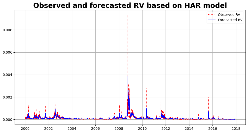

References

^Fulvio Corsi, A simple approximate long-memory model of realized volatility, Journal of Financial Econometrics 7(2) 174–196 (2009).
^Lan Zhang, Per A. Mykland and Yacine Aït-Sahalia, A tale of two time scales: Determining intergrated volatility with noise high-frequency data, Journal of the American Statistical Association, 100(472), 1394–1411 (2005).
^Bin Zhou, High-frequency data and volatility in foreign-exchange rates, Journal of Business & Economic Statistics, 14(1), 45–52 (1996).

Lecture Notes

Thanks to 刘弘锌 (Liú Hóng Xīn) for his lecture notes.

Moneyness: Moneyness (在值程度) 是金融衍生品中用于描述期权状态的核心概念, 它反映了期权的行权价 (Strike Price) 与标的资产当前价格 (Underlying Asset Price) 之间的关系.根据这种关系, 期权可以分为: 实值期权 (In-the-Money, ITM)、平值期权 (At-the-Money, ATM) 和虚值期权 (Out-of-the-Money, OTM).

In-the-Money: 行权后能获利.
At-the-Money: 行权后无利可图.
Out-of-the-Money: 行权后会亏损.

公式:

\[ \text{Moneyness} = \frac{K e^{-r \tau}}{S e^{-d\tau}}. \]

波动率理论基础与测算

核心定义与性质
- 多元定义本质: 波动率表征对数收益率的条件期望 $\sigma = \sqrt{\text{Var}(\log r_t)}$.
- 对数收益率优势: 时间可加性, 规避线性收益率跨期误差
- 微分规范: $\displaystyle \mathrm{d} (\log P_t) = \frac{\mathrm{d} P_t}{P_t} - \frac{1}{2}\left(\frac{\mathrm{d} P_t}{P_t}\right)^2$.
波动率的测算方法
- 滚动窗口法: 样本标准差 $\displaystyle s = \sqrt{\frac{1}{n-1} \sum_{i=1}^n (r_i - \bar{r})^2}$, 其中 $\bar{r}$ 为样本均值. 年度化波动率 $\sigma = s \sqrt{252}$.
- 窗口长度效应: 窗口长度 $n$ 越长, 波动率估计越平滑, 但反应速度较慢. 短窗口则更敏感, 但可能过度反应噪音.
分区理论应用
- 分区理论: 将时间序列分为多个区间, 每个区间内计算波动率, 以捕捉不同时间尺度的波动特征.
- 分区长度选择: 短期分区适合捕捉快速波动, 长期分区则更稳定. 例如, 5分钟、30分钟、日线等.

波动率特性与经典模型

波动率的特性
- 波动率聚集现象: 高波动率时期往往伴随高波动率, 低波动率时期则相反.
- 波动率微笑: 期权隐含波动率在不同执行价下呈现 U 形分布, 反映市场对不同风险的定价差异.
- 杠杆效应: 股价下跌时, 波动率往往上升, 反之亦然. 这与公司财务杠杆有关.
经典波动率模型
- 直接基于 Close Price 计算;
- Parkinson 模型: 基于最高价和最低价计算波动率, 适用于高频数据.
- Garman-Klass 模型: 结合开盘价、最高价、最低价和收盘价, 提供更精确的波动率估计.
- Yang-Zhang 模型: 进一步改进 Garman-Klass, 考虑了开盘价和收盘价的影响.

期权定价与市场情绪量化

定价模型
- Black-Scholes 模型: 基于几何布朗运动假设, 计算欧式期权价格.
- Heston 模型: 引入随机波动率, 更好地捕捉市场波动特性.
- Dupire 方程: 基于局部波动率假设, 计算期权隐含波动率曲面.
收益函数分解定理 \[ f(S_T) = f(K_0) + \int_{0}^{K_0} \frac{\partial^2 f}{\partial K^2} (K-S_T)^+ \mathrm{d}S + \int_S^\infty \frac{\partial^2 f}{\partial K^2} (S_T-K)^+ \mathrm{d}S, \] 通过期权组合复制任意连续收益.
市场情绪指标
- 未平仓量 (Open Interest): 反映市场参与者的情绪和预期. 看涨期权未平仓量增加通常表示市场对上涨的预期增强, 反之亦然.
- 交易量 (Volume): 期权交易量的变化可以反映市场情绪的变化. 例如, 看涨期权交易量增加可能表示市场对上涨的预期增强.
- 隐含远期预期: 近月 ATM 期权加权隐含收益率, 年化处理生成情绪指数.

关键公式总结

概念	公式	参数说明
对数收益率	\[r_t^{\log} = \ln(P_t/P_{t-1})\]	$P_t$: $t$ 时刻价格
年度化波动率	\[\sigma_{\text{annual}} = \sqrt{252} \times \hat{\sigma}_{\text{daily}}\]	252: 年交易日数
隐含远期价格	\[\hat{F} = K + e^{rT}(C - P)\]	$F$: 隐含远期价格
波动率微笑校准	\[\sigma_{\text{IV}}(K) = a + b\left(\frac{K-F}{F}\right)^2\]	$a$: ATM 波动率, $b$: 曲率

References

Carr, Peter, and Liuren Wu. 2004. “A Tale of Two Indices.” The Journal of Derivatives 13 (March). https://doi.org/10.2139/ssrn.871729.

Lecture 5: Volatility and volatility-linked derivatives

Agenda

What is volatility?

Why is volatility important?

Volatilities

Historical volatility

Example of historical volatility

Note

Exponentially weighted moving average (EWMA)

Now let’s dirty our hands …

Tips: You may skip the next 5 cells if you encounter an error.

You may start from here.

Volatility estimation using OHLC

Implied volatility

Why implied volatility rather than the price itself?

A practical tip for fetching risk free and dividend rates

Example - Implied volatilities of options on SPX

Tips: You may skip the next 12 cells if you encounter an error.

You may start from here

Create python class OptionAnalytics

A shorter time to expiry option on SPX

Tips: You may skip this part if you encounter an error.

You may start from here.

GPR fit for SPX implied volatility curve

Fine tune hyperparameters by MLE

What is VIX?

Volatility indices published by CBOE

Note

“Formula of financial engineering”

Remark

Example - log contract

Note

How is VIX calculated?

Download VIX data from yfinance

You may skip this part if you encounter an error.

Volatility derivatives

Variance swap

Volatility swap

Calculating volatility swap fair strike from MGF

VIX futures

VIX option

A look at the VIX option chain from Yahoo Finance

You may skip the next 5 cells if you encounter an error.

You may start from here.

GPR fit for VIX option implied volatility curve

Appendix (Optional)

Volatility estimation using high frequency data

Realized variance

Technical notes

Assumption

Integrated variance or quadratic variation

Note

Microstructure noise

Note

Asymptotic result

Note

The conventional solution

Subsampling

Boosting RV estimator

Note

The ZMA estimator

Note

The Zhou estimator

Realized library

Note

SPX realized variance

The Corsi HAR-RV forecast

Note

References

Lecture Notes

波动率理论基础与测算

波动率特性与经典模型

期权定价与市场情绪量化

关键公式总结

References

Create `python` class `OptionAnalytics`

Download VIX data from `yfinance`